Design of a supply chain to produce ethanol from one residuum and two coffee by-products
Bạn đang xem bản rút gọn của tài liệu. Xem và tải ngay bản đầy đủ của tài liệu tại đây (509.36 KB, 16 trang )
Uncertain Supply Chain Management 7 (2019) 767–782
Contents lists available at GrowingScience
Uncertain Supply Chain Management
homepage: www.GrowingScience.com/uscm
Design of a supply chain to produce ethanol from one residuum and two coffee by-products
Mónica Y. Castro-Peñaa*, César Augusto Peñuelab and Julián Gil Gonzálezc
a
Universidad Católica de Pereira, Pereira, Colombia
Universidad Libre, Pereira, Colombia
c
Universidad Tecnológica de Pereira, Pereira, Colombia
b
CHRONICLE
Article history:
Received November 4, 2018
Received in revised format
December 20, 2018
Accepted January 18 2019
Available online
January 18 2019
Keywords:
Residues
By-products
Coffee
Location
Ethanol
Supply chain
ABSTRACT
The present article exposes a model of Mixed Integer Linear Programming (MILP) as a support
for strategic decision making, guided to the location of facilities in ethanol supply chains under
a configuration of collection centers of raw material and production plants, directly impacting
costs related to logistics and operations. The model is applied to the supply chain for the
production of ethanol from two by-products and a coffee residue (pulp, mucilage, and stems,
respectively) in Colombia. The results obtained by the model allow identifying locations for
the corresponding links to the three types of biomass considered, and the flows of raw material
between coffee producing departments and collection centers, from the latter to production
plants, and from this, where the transformation of ethanol to mixing centers is generated.
© 2019 by the authors; licensee Growing Science, Canada.
1. Introduction
Recently, many studies have focused on the search for energetically efficient renewable energies to
minimize the negative impact on energy security generated by the use of fossil fuels and the reduction
of their reserves worldwide (Edenhofer et al., 2011). These sources of renewable energy must guarantee
industrial growth and the strengthening of the world economy (Zapiain, 1972); being biofuels one of
the most promising solutions.
Biofuels are classified into three categories according to the raw material used for their production. The
first generation comes from raw materials with a high content of starch, sugars, and oils (Alejos &
Calvo, 2015), which leads to an increased competition for land and water by using agricultural land for
the direct cultivation of biofuels, deforestation and the rise in the price of food (Hernández &
Hernández, 2008). The second generation makes use of lignocellulosic biomass from agricultural or
forestry residues (González Merino & Castañeda Zavala, 2008) listed as one of the best alternatives by
contributing to the reduction of land use due to its potential energy yield per hectare, not requiring
additional arable land to those that are used for human consumption (Loera-Quezada & Olguín, 2010).
* Corresponding author
E-mail address: (M. Y. Castro-Peña)
© 2019 by the authors; licensee Growing Science.
doi: 10.5267/j.uscm.2019.1.003
768
Finally, micro and macro algae are raw materials for the production of third generation biofuels through
the process of transesterification of the oils present in them (Martínez Restrepo, 2014); however, the
high costs generated by having controlled environments, the genetic engineering, together with the
production costs, means that this type of biofuel is at an incipient stage for commercial scale production
(Ecopetrol, 2014).
The above presents second-generation biofuels as a good option. However, the characteristics of its
raw material (lignocellulose) disadvantage its elaboration because it presents important technical
difficulties, which increases the cost of production and commercialization (Serna et al., 2011), making
the economic factor a limitation for its large-scale development. In this sense, the design of its supply
chain is identified as a critical factor for the reduction of operating costs (No, P. T., 2002).
In the context of supply chain management, several works are identified, which are mainly focused on
economic optimization, based on indicators such as: costs (Yue & You, 2014; Xie et.al., 2014; Emara
et al., 2016; Osmani & Zhang, 2017; Parker et al., 2010), earnings (Osmani & Zhang, 2017; Bai et al.,
2012), net present value (Kelloway et al., 2013), expected net present value (ENPV) formulated by
Bagajewicz, conditional value at risk (CVaR), and financial risk (Dal-mas et al., 2011). The latter is
analyzed from the different aspects that make up the operation of a supply chain for the generation of
biofuels such as location, the capacity of facilities, and flows of raw material (López-Díaz et al., 2017;
Sharifzadeh et al., 2015), technology for conversion (Leão et al., 2011; Kim et al., 2011), and aspects
guided to transportation decisions (Mohseni et al., 2016; Marvin et al., 2012). The above does not
ignore that the problem has been addressed from studies that have complemented the economic
indicators, also consider environmental (Natarajan et al., 2014; Mirkouei et al., 2016), environmental
and energetic (Zhang et al., 2012), and environmental and social aspects (Cambero & Sowlati, 2016).
Regarding the type of biomass used, contributions to corresponding biofuels of the three generations
are identified, being the most recorded biomasses in the search carried out as a case study: corn stubble,
forest residues, and switchgrass; only the article exposed by (Duarte et al., 2014) is identified, which is
closely related from the coincidence in the raw material of cut stems of coffee, and the context of the
country, Colombia. On the other hand, coffee is one of the most important agricultural products in
Colombia. The coffee sector is an essential contributor to GDP and a generator of employment in the
agricultural industry in the country (26% of total agricultural employment). Therefore, it is considered
as a real engine for the development of the rural economy and a "transcendental factor for sustaining a
social fabric that contributes directly to peace and rural development, reducing poverty, and boosting
production ..." (Lozano & Yoshida, 2008) The country, as of September 2017, had a "coffee park that
exceeds 4,700 million trees distributed over more than 911,000 hectares in 600 municipalities"
(Federación Nacional de Cafeteros, 2017). Nonetheless, coffee plants generate large volumes of
organic residues. In fact, only 5% of the weight of the fresh fruit is used in the preparation of the coffee
drink (Serna-Jiménez et al., 2018). Usually, coffee residues are thrown into streams, a fact that causes
contamination of water sources, which leads to the death of aquatic species (Funes et al., 2011). The
residues and by-products of coffee can be used as fuel in different ways including: as a direct fuel,
biogas, biodiesel, and bioethanol (fuel alcohol); in the case of bioethanol, studies such as Triana et al.
(2011), Navarro et al. (2017), Muñoz & Daniel (2015), Navia et al. (2011) and Gurram et al. (2015)
have demonstrated and studied the process under which stems, mucilage, and fresh pulp can be raw
material for the production of fuel alcohol.
In this way, the present article exposes the development of a Mixed Integer Linear Programming model
(MILP) as a support for strategic decision making guided to the location of facilities in ethanol supply
chains, under a configuration of centers of raw materials and production plants. The present model
considers restrictions of availability of raw material, taking as a reference the model of
location/assignment, Location-Allocation Problem (LAP), which is a combinatorial problem that
consists of determining the position of k facilities on possible positions and assigning customers to the
nearest facility (Torrent-Fontbona et al., 2013). The LAP is considered in the literature as a NP-hard
problem (Zurita-Milla & Huisman, 2011), which requires a solution methodology that faces the
M. Y. Castro-Peña et al. /Uncertain Supply Chain Management 7 (2019)
769
computational complexity, and results can be obtained in reasonable execution times. As a case study,
the supply chain for the production of ethanol is taken from two by-products (pulp, mucilage), and a
coffee residue (stems) in Colombia. This country has 1,102 municipalities, of which 600 are coffee
producers (Federación Nacional de Cafeteros, 2017); being considered as the largest producer of soft
washed Arabica coffee in the world, and which production grew 83% in the last four years (Federación
Nacional de Cafeteros de Colombia, 2016).
2. Structure and development of the model
The development of the proposed model tends for a design of a supply chain for the production of
ethanol from three second-generation raw materials, being these by-products and residues of coffee;
the design is carried out according to the scheme shown in Fig. 1, in which the links that will make up
the chain belonging to the pulp biomass are shown, for the case of mucilage and stems it will be the
same, varying the subscripts used for each case (Table 1). The links considered for the supply chain are
four: coffee producing departments, raw material collection centers, production plants, and mixing
centers. Two (2) of these links already have a defined location, coffee-producing departments, and
mixing centers, being the object of study and purpose of the model to be proposed, establishing the
location of collection centers and production plants, as well as determining the flow between them once
their location is defined.
Fig. 1. Scheme of the proposed supply chain.
Table 1
Subscripts used in the model
Set
єJ
єD
єF
єU
єL
єZ
єG
єE
єO
єP
єN
єC
єI
єK
єA
єM
єW
Description
Set of departments suppliers of pulp biomass
Set of departments suppliers of mucilage biomass
Set of departments suppliers of stems biomass
Set of location alternatives for mucilage collection centers
Set of location alternatives for pulp collection centers
Set of alternatives for zoca collection centers
Set of mucilage collection centers
Set of zoca collection centers
Set of pulp collection centers
Set of location alternatives for pulp production plants
Set of location alternatives for mucilage production plants
Set of location alternatives for zoca production plants
Set of mucilage processing plants
Set of zoca processing plants
Set of pulp processing plants
Set of available mixing centers
Ethanol
770
The problem is formulated as a Mixed Integer Linear Programming model, taking as reference the
parameters shown in Table 2 for the establishment of the optimal values for the decision variables
indicated in Table 3.
Table 2
Parameters
Symbol
CBDG
CBJO
CBFE
CBGI
Cost of mucilage transport from collection center
production plant located in region
CBOA
Cost of pulp transport from collection center
production plant located in region
CBEK
CEIM
CEAM
CEKM
TPP
TPM
TPZ
CBP
CBM
CBZ
QP
QM
QZ
CFVO
CFVE
CFVG
CFVA
CFVK
CFVI
DM
QCA
QCK
QCI
QAO
QAE
QAG
CDNS
Description
Cost of mucilage transport from department to collection center located in
region
Cost of pulp transport from department to collection center located in
region
Cost of zoca transport from department to collection center located in region
located in region
to the
located in region to the
Cost of zoca transport from the collection center located in region to the
production plant located in region
Cost of ethanol transport from the production plant located in region to the
mixing center
Cost of ethanol transport from the production plant located in region to the
mixing center
Cost of ethanol transport from the production plant located in region to the
mixing center
Ethanol production rate from pulp
Ethanol production rate from mucilage
Ethanol production rate from stems
Cost of pulp raw material in region
Cost of mucilage raw material in region
Cost of stems raw material in region
Amount of pulp available in department
Amount of mucilage available in department
Amount of stems available in department
Fixed and variable costs of opening of collection center located in region
Fixed and variable costs of opening of collection center located in region
Fixed and variable costs of opening of collection center located in region
Fixed and variable costs of opening of production plant located in region
Fixed and variable costs of opening of production plant located in region
Fixed and variable costs of opening of production plant located in region
Ethanol demand by the mixing center
Conversion capacity of the production plant in the region
Conversion capacity of the production plant
Conversion capacity of the production plant
Storage capacity of the collection center in the location
Storage capacity of the collection center in the location
Storage capacity of the collection center in the location
Unmet demand cost in the mixing center
Unit
$/ton
$/ton
$/ton
$/ton
$/ton
$/ton
$/Lt
$/Lt
$/Lt
Lt/ton
Lt/ton
Lt/ton
$/ton
$/ton
$/ton
Ton/mes
Ton/mes
Ton/mes
$
$
$
$
$
$
Lt/mes
Lt/mes
Lt/mes
Lt/mes
Ton/mes
Ton/mes
Ton/mes
$/Lt
771
M. Y. Castro-Peña et al. /Uncertain Supply Chain Management 7 (2019)
Table 3
Decision variables
Symbol
Description
1 if the production plant is established at location ; otherwise 0
YI
1 if the production plant is established at location ; otherwise 0
YK
1 if the production plant is established at location ; otherwise 0
YA
1 if the collection center is established at location ; otherwise 0
YG
1 if the collection center is established at location ; otherwise 0
YE
1 if the collection center is established at location ; otherwise 0
YO
Amount of pulp transported from department to the collection center located
XJ
in region
Amount of stems transported from department to the collection center
XF
located in region
Amount of mucilage transported from department to the collection center
XD
located in region
Amount of pulp sent from the collection center located in region to the
XBO
production plant located in region
Amount of mucilage sent from the collection center located in region to the
XBG
production plant located in region
Amount of stems sent from the collection center located in region to the
XBE
production plant located in region
Amount of ethanol to be sent from the production plant located in region to
XEA
the mixing center
Amount of ethanol to be sent from the production plant located in region to
XEI
the mixing center
Amount of ethanol to be sent from the production plant located in region to
XEK
the mixing center
Total ethanol generated from mucilage by the plant located in region
XBM
Total ethanol generated from pulp by the plant located in region
XBP
Total ethanol generated from stems by the plant located in region
XBZ
Slack variable to satisfy the demand restriction of the mixing center
XVIRT
Unit
[0,1]
[0,1]
[0,1]
[0,1]
[0,1]
[0,1]
Ton.
Ton.
Ton.
Ton.
Ton.
Ton.
Lt
Lt
Lt
Lt
Lt
Lt
Lt
According to the information presented as a basis for the formulation of the model, each of its
components is related in the following sections.
2.1 Objective function
This function is determined by the minimization of costs (eq. 1) by concept in the first measure of
transport between the different links, as well as from the first to the third component of multiplication
obey said cost between suppliers and collection centers, the following three to transport between
collection centers and production plants, and from the seventh to the ninth component to the transfer of
ethanol to the respective mixing centers. The other costs involved correspond to fixed and variable
costs due to the opening of both collection centers (component 10 to 12), and production plants
(component 13 to 15); finally, a penalty for unmet demand is considered.
772
∗
∈
∈
∈
∈
∈
∈
∈
∈ ∈
∗
∈
∈
∗
∗
∈
∈
∗
∈
∈
∈
∗
∗
∈
∗
∈
∈
∈
∗
∈
∗
∈
(1)
∈
∈
∈
∈
∈
∗
∈
∗
∈
∈
∗
∈
∗
∈
∈
∈
∈
∈
∗
∈
∈
∈
∈
∈
∗
∈
∈
2.2 Model constraints
The eq. (2) - (37) presents the restrictions of the proposed model for link location effects. The first set
of restrictions, eq. (2) - (11), ensures the non-negativity of the related variables.
;∀ ∈ ;∀ ∈ ;∀ ∈
(2)
;∀ ∈ ;∀ ∈ ;∀ ∈
;∀ ∈
(3)
;∀ ∈ ;∀ ∈
(4)
;∀ ∈ ;∀ ∈ ;∀ ∈ ; ∀ ∈
(5)
;∀ ∈ ;∀ ∈ ;∀ ∈ ; ∀ ∈
(6)
;∀ ∈ ;∀ ∈ ;∀ ∈ ; ∀ ∈
(7)
;∀ ∈ ; ∀ ∈ ;∀
(8)
;∀ ∈ ;∀ ∈ ;∀
;∀ ∈ ; ∀ ∈ ;∀
;∀
∈
∈
∈
(9)
∈
(10)
(11)
The second block of equations is given by eq. (12) - (21), which are established for each of the three
subjects considered in the model, and will be exemplified with those corresponding to the pulp. The
restriction represented in the Eq. (12) ensures that the available biomass is collected.
∀ ∈
∈
(12)
∈
This biomass collected and sent, according to its type, to the collection center and subsequently to the
corresponding production plant, cannot exceed the storage capacity of these links for each of the raw
materials, as restricted by the Eqs. (13-14) respectively.
773
M. Y. Castro-Peña et al. /Uncertain Supply Chain Management 7 (2019)
∗
∀ ∈ ;∀ ∈
(13)
∈
∗
∀ ∈ ; ∀ ∈
(14)
∈
Regarding the collection centers, the Eq. (15) determines that each of these, for the raw materials
considered, are unique; therefore, they may be established in only one of the given location alternatives.
Likewise, in order to have a higher coverage, it is determined that of the group of possible collection
centers of each of the raw materials, each one of these should be opened in alternatives of different
location, that is, there cannot be two collection centers for the same raw material in the same location
(Eq. 16).
∀ ∈
(15)
∀ ∈
(16)
∈
∈
The Eq. (17) works as a transshipment, determining that the amount of raw material sent from each
collection center to the production plants must be equal to the quantity received by each collection
center from the different biomass suppliers departments. In the same way that happens with ethanol
(product of the conversion of biomass) generated by each of the production plants, it must be sent in
its entirety to the respective mixing centers, as defined by Eq. (18).
∀ ∈ ; ∀ ∈
∈
∈
(17)
∈
∀ ∈ ;∀
∈ ;∀
∈
(18)
∈
Each of the components of the set of production plants of the raw materials considered can be located
in only one of the location alternatives. That is, a specific production plant cannot be assigned in more
than one location, as expressed by Eq. (19). In addition, the Eq. (20) establishes that in each of the
location alternatives for these links can be established a maximum of one, for certain raw material.
∀ ∈
(19)
∀ ∈
(20)
∈
∈
Once each of the biomasses is in their respective production plants, the amount that enters is multiplied
by the conversion rate, being the product equivalent to the total ethanol generated; said transformation
is represented by the Eq. (21).
∀ ∈ ;∀ ∈ ;∀
∗
∈
∈
(21)
∈
The Eq. (22) indicates that what is sent from the production plants to the mixing centers, responds to a
demand that is generated in each one of these. A virtual variable is added in this restriction so that it
takes the value of the remaining or missing ethanol with respect to the demand.
∈
∈
∈
∈
∀
∈
∈
∈
(22)
774
Finally, the set of equations Eqs. (23-37) are established to avoid nonlinearity in the model, taking as a
reference the variables that represent the flows generated between different links, using the Big M
method.
∗
∀ ∈ ; ∀ ∈ ; ∀ ∈
(23)
∗
∀ ∈ ; ∀ ∈ ; ∀ ∈ ; ∀ ∈
(24)
∗
∀ ∈ ; ∀ ∈ ; ∀ ∈ ; ∀ ∈
(25)
∗
∀ ∈ ; ∀ ∈ ; ∀
∈
(26)
∗
∀ ∈ ; ∀ ∈ ; ∀
∈
(27)
∗
∀ ∈
∗
∗
;∀ ∈ ;∀ ∈
∀ ∈ ; ∀ ∈ ; ∀ ∈ ; ∀ ∈
∀ ∈ ; ∀ ∈ ; ∀ ∈ ; ∀ ∈
(28)
(29)
(30)
∗
∀ ∈ ; ∀ ∈ ; ∀ ∈
(31)
∗
∀ ∈ ; ∀ ∈ ; ∀
(32)
∗
∈
∀ ∈ ; ∀ ∈ ; ∀ ∈
(33)
∗
∀ ∈ ; ∀ ∈ ; ∀ ∈ ; ∀ ∈
(34)
∗
∀ ∈ ; ∀ ∈ ; ∀ ∈ ; ∀ ∈
(35)
∗
∀ ∈ K; ∀ ∈ C; ∀
∈M
(36)
∗
∀ ∈ K; ∀ ∈ C; ∀
∈W
(37)
Under the above restrictions, the location for collection centers of the three raw materials considered is
determined, as well as their respective production plants. Thus, with this information, it is proceeded
to determine the flows that are generated between the links, for which the model already exposed is
taken as a base, with the opening binary variables and the sub-indices of location alternatives being
eliminated, therefore, the components of the objective function and restrictions that refer to these
aspects.
3. Case study
3.1. Determination of elements of the sub-index sets
The model is applied in Colombia, taking as a database for the possibilities of the corresponding link
to coffee producing departments, those presented by (Federación Nacional de Cafeteros de Colombia,
2016) and representing a percentage equal or greater than 3% of cultivated coffee area; thus, the 13
selected departments represent 95% of the cultivated area in this country. In order to reduce the
computational complexity of the mathematical model, they are grouped into 3 conglomerates (zones),
and so, define a smaller number of location alternatives for collection centers and production plants.
Through the implementation of the k-means algorithm (MacQueen, 1967), fed with the coordinates of
the cities of the departments under study, which also determines the centroid or midpoint for each of
the zones. These points are taken as alternative locations for collection centers, by geographical criteria
and distance terms. Next, the generated zones are exposed, and the centroid of each of these is
highlighted:
Zone 1: Cesar, Norte de Santander, Santander.
Zone 2: Antioquia, Caldas, Cundinamarca, Quindío, Risaralda, Tolima.
M. Y. Castro-Peña et al. /Uncertain Supply Chain Management 7 (2019)
775
Zone 3: Cauca, Huila, Nariño, Valle.
After analyzing that in zone 1, the raw material produced by 11% of thousands of hectares cultivated
in the country would be collected, while from zones 2 and 3 they would collect the corresponding to
47% and 37% respectively, an alternative is proposed additional to the midpoints for each of the last
two named zones, the selection criterion being the volume of cultivated area. In this way, for zone 2,
the reference point selected for production is Antioquia, and for zone 3 Huila.
Hence, the five departments taken as reference points (Norte de Santander, Tolima, Antioquia, Cauca,
Huila) are those that are taken as alternatives in the mathematical model for the location of collection
centers and production plants for the different raw materials. Likewise, factors that are considered
(Duarte et al., 2013) as incidents in the location of facilities are analyzed, among which the agricultural
capacity, the quality of the transportation infrastructure, the attitude of the community towards a
project, the social impact of the region, the living conditions, and safety and criminality are named.
This analysis is carried out based on information available in the document "Coffee Regional
Competitiveness Index" (Lozano & Yoshida, 2008).
Regarding the link “mixing centers”, in Colombia these are already established, also known as
“wholesale distributors”; the first reference is the “List of agents of the fuel distribution chain”
(Ministerio de minas y energía, 2012), from which the purposes of the present study were selected,
specifically those dedicated to the ethanol mixture, enunciated in resolutions number 4-0717 of 2016,
and 9-0153 of 2014 of MinMinas, in which wholesale supply plants of specific areas dedicated to make
mixtures called "E-8" (8% fuel alcohol with 92% motor gasoline) are established.
According to the above, a list of 38 mixing centers is obtained, which are grouped according to the
department where they are located, concluding a total of 16 departments; however, for the purposes of
the parameters of the model, for each of these, the distance from the possible locations of production
plants should be calculated, a process that was not possible using the tool used (Google maps), for the
departments of Amazonas and Guainía, so that, for the purposes of this study, reference will be made
to the 14 remaining departments.
What has been said so far regarding the determination of sub-index is summarized in Table 4, where
reference is made to the set and description of these and to the specific elements that have been selected
based on the reality represented by the selected country as a case study.
Table 4
Equivalence of sub-index in the case study
Set
Description
Set of selected biomasses
∈ B
Set of biomass supplier
∈J
departments
∈U
∈ P
∈ M
Set of alternatives for the location
of collection centers
Set of alternatives for the location
of production plants
Set of available mixing centers
Source: The authors.
Elements
[stems, mucilage, pulp]
[Antioquia, Caldas, Cauca, Cesar, Cundinamarca,
Huila, Nariño, Norte de Santander, Quindío,
Risaralda, Santander, Tolima, Valle]
[Norte de Santander, Tolima, Antioquia, Cauca,
Huila]
[Norte de Santander, Tolima, Antioquia, Cauca,
Huila]
[Cundinamarca, Risaralda, Valle, Tolima, Huila,
Caldas, Caquetá, Putumayo, Vichada, Guaviare,
Bolívar, Atlántico, Santander, Antioquia,
Sobrante]
776
3.2. Determination of parameters
Regarding the calculation of transport costs between the different links, it is based on the "Table of
minimum economic relations between the transport company and the owner of the linked vehicle"
(Ministerio de transporte, 2007), in which the value per ton transported between certain origins and
destinations is exposed, in the event that these points are not specified in the table, the fourth paragraph
of the second article of resolution 3175 of August 1, 2008 states that the value to be paid per ton will
be determined as the reference route the nearest origin that is in said table.
With this figure and the average distances between the departments and location alternatives for the
collection centers, the average transport value of ton per kilometer is determined, which in turn is
divided by the respective distance between links, leaving them described in units of $/ton; this value is
designated for transport costs corresponding to the stem raw material since it does not require any
treatment; otherwise, the mucilage and the pulp must be under certain thermal conditions to avoid
fermentation by natural means, so the transport cost of these biomasses is added an additional value for
the concept of necessary refrigeration.
The costs related to the transportation of ethanol as a final product to the different mixing centers are
calculated according to an average rate of those given by the Ministry of Mines and Energy (Ministerio
de Minas y Energía, 2005), specific for the transport of alcohol fuel between distillers and plants of
supply wholesalers.
Concerning the availability of raw material in the selected departments as alternatives of suppliers in
the present project, a limitation is evident from the lack of information; therefore, the data that are taken
for validation are calculated according to figures presented in thousands of hectares by department
registered until September of 2015 by the FNC. The percentage of participation of each of the
departments is calculated on the national production, which is uniformly distributed in the months that
according to information presented by Asoexport (s.f.), are the periods of coffee harvest in the different
departments of the Colombian territory; later, this is converted to its value in thousands of hectares that
would be harvested per month in each of the departments. With this information, we go to the average
productivity value of Colombian coffee, which exceeds 15.4 bags of 60 kilograms of green coffee per
hectare, (Federación Nacional de Cafeteros de Colombia, 2016), and once having the figures in these
units, it is proceeded to make use of calculations carried out by Rodríguez (2015), where they explain
that for every million bags of green coffee produced, pulp and fresh mucilage are generated, 162,900
and 55,500 tons respectively, thus establishing the tons of mucilage and pulp generated by each of the
departments in the different months of the year.
In the case of stems, the number of hectares per type of work (sowing renewal and zoca renewal) is
available in each of the months of 2014 by the coffee producing departments (Federación Nacional de
Cafeteros, 2015); in the same way, it is determined that in average per hectare, 16 tons are obtained,
using this figure as a conversion factor to establish the total of tons of stems available in each of the
departments selected as suppliers of raw material in each of the months.
In relation to the ethanol production rates, one ton of pulp yields 25.17 liters of ethanol and 58.37 liters
of mucilage (Rodríguez, 2015). In the case of stems, a yield of 240 liters per ton is obtained (Triana et
al., 2011). The raw materials considered in this study have not yet been commercialized; hence, they
do not have an established cost for their sale, according to this, the value given for the ton of stems in
the study is taken as reference for the present study (Duarte et al., 2014) because the geographic and
social context taken in this is the same.
Respecting the demand for ethanol by each of the departments with mixing centers considered and
exposed in Table 9, reference is made to the information concentrated in the "Balance of the Colombian
sugar sector 2000 - 2016" (Fondo de Estabilización de precios del Azúcar (FEPA), 2016) where the
production and sales to the national market are exposed for ethanol in thousands of liters. Taking into
account that the final link considered in the present study are the mixing centers and that these must
777
M. Y. Castro-Peña et al. /Uncertain Supply Chain Management 7 (2019)
supply the national demand for ethanol required, the thousands of liters sold to the national market in
the months of 2015 are taken, since those of 2016 are subject to changes by the FEPA audit.
The capacities for both, collection centers and conversion plants, are calculated according to the
maximum production per month that will have each of the types of raw material considered in the
present investigation. Taking into account that the model takes as a maximum number to be established
three, the production is divided among these; and with respect to the conversion plants that are available
for each raw material, the maximum amount of ethanol produced per month is calculated, giving this
value its maximum capacity.
Finally, the fixed and variable opening costs for both collection centers and production plants will not
be introduced within the present validation; however, the parameter is left established in the model for
future application cases. The foregoing is due to the fact that, in reviews of the current literature, no
data is recorded that can serve as a reference for establishing the value of these parameters. Therefore,
the installation decisions generated from the present validation respond to the minimization of costs for
transport and value of raw material collected, in costs related to opening, the variable "zero" is taken
as the value due to that there are not enough criteria to be established, or differentiated by zones; the
other option is generated by assuming non-zero values that are the same for all alternatives, however,
since there are no differentiating values, the opening decisions are the same as by assuming a value of
zero.
4. Results and analysis
The proposed model, both for identification of locations and for the manager of flow optimization, was
developed by means of the GAMS Software (General Algebraic Modeling System), version 21.2,
executing the CPLEX algorithm for its solution, being good the computational times presented.
4.1. Identification of locations
This first model consists of 47 blocks of equations, 20 blocks of variables, 6535 non-zero elements,
1527 individual equations, 1151 individual variables and 60 discrete variables, which was executed for
each of the months of the year (12 times), varying in each of these, the amount of raw material available
in the departments selected as suppliers, and the quantity of ethanol demanded in this same unit of time
in the departments that own the mixing centers (wholesale distributors). The above, in order to analyze
the stability of the location of the collection centers and production plants with respect to the variations
made; thus, the most stable location options before the climate dynamics that condition the crops and
good practices in these, and the demand for ethanol in the different months of the year in Colombia,
are inputs for the optimization of flows between the different links of the supply chain.
For purposes of the collection centers, it is proposed in the model that a maximum of three (3) are
generated for each type of raw material, so that any of these can be opened according to the conditions
that are generated. Table 5 shows a count of the times that the location alternatives are selected for this
opening.
Table 5
Counting collection center locations
Location
Norte de Santander
Antioquia
Tolima
Cauca
Huila
Pulp
2
5
8
4
6
Raw material
Mucilage
1
4
8
7
5
Stems
0
5
11
9
4
Total openings
3
14
27
20
15
778
It is evident that, for the three raw materials, the alternative of location with more openings in the
different months is Tolima. For the case of mucilage and stems the second alternative to select is Cauca,
and Huila for pulp, finding the numbers of months in which the opening is made with a significant
difference compared to the other options; the situation is different for the selection of a third center of
collection, because the difference in the number of months that is opened is not significant, so the total
openings of the locations is taken as the second selection criterion because said value represents greater
stability, so the third location for the collection center of mucilage and stems is Huila, and for the
collection of pulp it will be Cauca. According to the above, the locations of the collection centers for
each of the raw materials coincide in the departments of Tolima, Cauca and Huila.
In regard to the location of production plants, table 6 is presented, where a count is carried out that
clearly allows identifying Tolima as the most optional department for the establishment of the ethanol
production plant from the biomass corresponding to the pulp and stems, being the difference with the
rest of options of location equal or superior to 3 months; nonetheless, for the case of mucilage, the
location that the production plant must have for its treatment is not completely clear, which is why a
second criterion equal to that of the selection of collection centers (selected location in a greater number
of months in general) is considered, being the department of Tolima selected for the processing of the
mucilage, and not Huila as it would be concluded by the information presented in Table 6 due to its
little differentiation with respect to the rest of the departments, and the proximity presented with
Tolima, which according to the second criterion is the one selected, being these neighboring
departments.
Table 6
Counting production plants locations
Location
Norte de Santander
Antioquia
Tolima
Cauca
Huila
Pulp
2
1
5
1
2
Raw material
Mucilage
0
2
2
3
4
Stems
0
2
8
1
1
Total months with openings
2
5
15
5
7
According to the information presented, it is concluded that both collection centers and production
plants would share locations. Cauca and Huila are the locations for the collection centers, in addition
to Tolima, department that also appears as the best option for the establishment of production plants
for the processing of the three biomasses, so it could be concluded that it is convenient the construction
of a multi-plant for the production of ethanol from mucilage, pulp, and stems, taking into account that
in the month of July, it would only process stems.
4.2. Flows optimization
It is carried out using the model initially proposed with the modifications referring to the elimination
of location alternatives, and hence, open binary variables, consisting of 20 blocks of equations and 14
variables, 669 non-zero elements, 82 individual equations, and 199 different variables.
According to the flows, there are times of the year in which collection centers for certain biomass can
be inactivated due to the little or no existing quantity of these in the coffee producing departments,
linked to the period of the main harvest, “mitaca”, crop renovations or implementation of good
practices, as shown in Table 7.
779
M. Y. Castro-Peña et al. /Uncertain Supply Chain Management 7 (2019)
Table 7
Activity of collection centers by flows
Location
Tolima
Cauca
Huila
Biomass
Mucilage
Number of inactive months
2
Pulp
2
Stems
Mucilage
0
5
Pulp
5
Stems
Mucilage
0
6
Pulp
6
Stems
8
Active Periods
March – June
August - January
March – June
August - January
January – December
Nov.-February
April-June
Nov.-February
April-June
January – December
April-June
October – Dic.
April-June
October – Dic.
January-March
June
It can be evidenced that the collection centers of stems located in Tolima and Cauca are the only ones
that must be enabled throughout the year for the reception of raw material, leading to the one located
in Huila for the reception of this matter to be that of a minor activity in the year, against which decisions
could be made due to the proximity it has with the department of Tolima.
On the other hand, collection centers for pulp and mucilage have the same activity, being logical to be
both by-products of the production of coffee beans, namely dependent on the same source. Following
the order of the flow of the raw material, the tons sent from the collection centers to production plants
is the same as that received by each of the collection centers due to the restriction that makes them
operate as a transshipment node, meaning that the only month in which the ethanol plants from
mucilage and pulp will be completely inactive is July, since the production of the coffee bean for this
month is null.
Lastly, according to the flows generated from the production plants to the mixing centers, it is evident
that there are months with a surpass to the demanded amount of ethanol (January and May), which
could be considered for export, or in its effect for the generation of reserves for the national market as
there are months in which the production of ethanol does not fully meet the demand of the departments.
Table 8 shows more precisely the 14 mixing centers selected for the validation of the model, how many
of these are served in a complete (AC), partial (AP) or null (NA) manner, as well as the liters of fuel
alcohol missing to meet the national demand in each of the months.
Table 8
Attention to mixing centers
AC
January
February
March
April
May
June
July
August
September
October
November
December
14
11
8
11
14
10
5
6
5
6
4
4
Mixing centers
AP
NA
1
2
1
5
1
2
1
3
1
8
1
7
1
8
1
7
1
9
10
Missing Liters
(Millions)
5,08
9,93
3,95
2,50
22,0
15,4
24,3
15,4
18,0
27,0
Remaining Liters
(Millions)
16,9
3,38
-
780
5. Conclusions
In the pre-modeling phase, it is established that the raw material selected for the present supply chain
is highly striking for the yields generated in the production of fuel alcohol, especially the stems that
represent a comparatively high yield with the by-products of coffee, in addition to requiring less care
during the production process since the risk of fermentation by natural means is not generated with this
residue; thence, it does not require refrigeration temperatures, being in turn the treatment of this less
expensive. However, the characteristics established in previous studies, regarding the mucilage and the
pulp, allow these to be considered within this research.
Under the approach taken in the present research based on the variability of availability of coffee byproducts (pulp and mucilage), and the stems as residue that is generated, the facility location model
allows to establish locations according to the selected reality as a case study, in computationally good
times.
The validation of the performance of the model had two phases, the first where the locations for
collection centers and production plants are established, and the second, the optimization of flows. In
the first phase, it is concluded that the locations that favor the variability of availability of raw material
is shared by the three types of biomass considered, this is how the locations for collection centers for
both by-products and residue are the same (Tolima, Cauca, and Huila), and in the case of production
plants, the three have to be in the department of Tolima, this location coinciding with the only article
related directly and in the same Colombian context to the present investigation (Duarte et al., 2014).
Future works
As a topic for future research, it is proposed that due to the location generated for collection centers
and production plants, costs are calculated as multipurpose locations, where the three types of raw
material are received and processed.
On the other hand, in the present investigation, the periods of time (months) were analyzed separately;
for this reason, it is proposed to generate a single model where all the months of the year are considered
as a variable, and to make a comparison of the variation of results for both, location and flows.
References
Alejos, C., & Calvo, E. (2015). Biocombustibles de primera generación. Revista Peruana de Química
e Ingeniería Química, 18(2), 19-30.
Asoexport. (s.f.). />Bai, Y., Ouyang, Y., & Pang, J. S. (2012). Biofuel supply chain design under competitive agricultural
land use and feedstock market equilibrium. Energy Economics, 34(5), 1623-1633.
Cambero, C., & Sowlati, T. (2016). Incorporating social benefits in multi-objective optimization of
forest-based bioenergy and biofuel supply chains. Applied Energy, 178, 721-735.
Dal-Mas, M., Giarola, S., Zamboni, A., & Bezzo, F. (2011). Strategic design and investment capacity
planning of the ethanol supply chain under price uncertainty. Biomass and bioenergy, 35(5), 20592071.
Duarte, A. E., Sarache, W. A., & Costa, Y. J. (2014). A facility-location model for biofuel plants:
Applications in the Colombian context. Energy, 72, 476-483.
Duarte, A. E., Sarache, W. A., & Matallana, L. G. (2013). Incident factors in facility location: An
application in the Colombian biofuel sector. Ingeniería e Investigación, 33(3), 72-75.
Ecopetrol.
(2014).
Biocombustibles.
/>Edenhofer, O., Pichs-Madruga, P. M., & Sokona, Y. (2011). Fuentes de energía renovables y mitigación
del cambio climático. Informe Especial del GRUPO Intergubernamental de expertos sobre el
Cambio Climático.
M. Y. Castro-Peña et al. /Uncertain Supply Chain Management 7 (2019)
781
Emara, I. A., Gadalla, M. A., & Ashour, F. H. (2016). Supply chain design network model for biofuel
and petrochemicals from biowaste. Chemical Engineering Transactions, 52, 1069-1074.
Federación Nacional de Cafeteros (2015). Sistema de Información Cafetera SICA. Disponible en:
/>cion_sica-1/
Federación Nacional de Cafeteros de Colombia. (2016). Informe del comportamiento de la industria
2015. eracion de
cafeteros.org/static/files/Informe_Comportamiento_de_la_Industria_2015.pdf.
Federación Nacional de Cafeteros de Colombia. (2016). Colombia cerró 2015 con cosecha cafetera
récord en los últimos 23 años. />Federación Nacional de Cafeteros (2017). Productividad alcanza 18.7 sacos , un salto de 32%. 85°
Congreso Nacional de cafeteros. Disponible en:
/>Fondo de Estabilización de precios del Azúcar. (2016). Balance azucarero mensual ASOCAÑA.
/>González Merino, A., & Castañeda Zavala, Y. (2008). Biocombustibles, biotecnología y alimentos:
Impactos sociales para México. Argumentos (México, DF), 21(57), 55-83.
Gurram, R., Al-Shannag, M., Knapp, S., Das, T., Singsaas, E., & Alkasrawi, M. (2016). Technical
possibilities of bioethanol production from coffee pulp: a renewable feedstock. Clean Technologies
and Environmental Policy, 18(1), 269-278.
HERNáNDEZ, M., & Hernández, J. (2008). Verdades y mitos de los biocombustibles. Elementos, 71,
15-18.
Kelloway, A., Marvin, W. A., Schmidt, L. D., & Daoutidis, P. (2013). Process design and supply chain
optimization of supercritical biodiesel synthesis from waste cooking oils. Chemical Engineering
Research and Design, 91(8), 1456-1466.
Kim, J., Realff, M. J., Lee, J. H., Whittaker, C., & Furtner, L. (2011). Design of biomass processing
network for biofuel production using an MILP model. Biomass and bioenergy, 35(2), 853-871.
Leão, R. R. D. C. C., Hamacher, S., & Oliveira, F. (2011). Optimization of biodiesel supply chains
based on small farmers: a case study in Brazil. Bioresource technology, 102(19), 8958-8963.
Loera-Quezada, M., & Olguín, E. J. (2010). Las microalgas oleaginosas como fuente de biodiesel: retos
y oportunidades. Rev. Latinoam. Biotecnol. Amb. Algal, 1(1), 91-116.
López-Díaz, D. C., Lira-Barragán, L. F., Rubio-Castro, E., Ponce-Ortega, J. M., & El-Halwagi, M. M.
(2017). Optimal location of biorefineries considering sustainable integration with the
environment. Renewable Energy, 100, 65-77.
Lozano, A., & Yoshida, P. (2008). Índice de competitividad regional cafetero. Revista Ensayos sobre
economía cafetera, 24.
MacQueen, J. (1967, June). Some methods for classification and analysis of multivariate observations.
In Proceedings of the fifth Berkeley symposium on mathematical statistics and probability(Vol. 1,
No. 14, pp. 281-297).
Martínez Restrepo, J. M. (2014). Selección de hongos filamentosos con potencial para la degradación
de lignocelulosa aislados de desechos agroindustriales de café e higuerilla.
Marvin, W. A., Schmidt, L. D., & Daoutidis, P. (2012). Biorefinery location and technology selection
through supply chain optimization. Industrial & Engineering Chemistry Research, 52(9), 31923208.
Ministerio de Minas y Energía. (2012). Agentes de la cadena.
/>+30-2012.pdf/89d639f4-5515-4370-8614-93b6df3d5a87.
Ministerio de Minas y Energía. (2005).
Ministerio de Transporte. (2007). Resolución No. 000888.
782
Mirkouei, A., Mirzaie, P., Haapala, K. R., Sessions, J., & Murthy, G. S. (2016). Reducing the cost and
environmental impact of integrated fixed and mobile bio-oil refinery supply chains. Journal of
cleaner production, 113, 495-507.
Mohseni, S., Pishvaee, M. S., & Sahebi, H. (2016). Robust design and planning of microalgae biomassto-biodiesel supply chain: A case study in Iran. Energy, 111, 736-755.
Muñoz, G., & Daniel, C. (2015). estandarización de producción de bio-etanol a base de mucilago de
café en la planta de biocombustibles del tecno-parque Yamboro del Sena Pitalito Huila.
No, P. T. (2002). Marco conceptual de la cadena de suministro: un nuevo enfoque logístico.
Natarajan, K., Leduc, S., Pelkonen, P., Tomppo, E., & Dotzauer, E. (2014). Optimal locations for
second generation Fischer Tropsch biodiesel production in Finland. Renewable Energy, 62, 319330.
Navarro, S. L. B., Castillo, B., & López, A. L. (2017). Validación del mucílago de café para la
producción de etanol y abono orgánico. El Higo Revista Científica, 3(1), 10-13.
NAVIA, D. P., VELASCO, R. D. J., & HOYOS, J. L. (2011). Production and evaluation of ethanol
from coffee processing by-products. Vitae, 18(3), 287-294.
Osmani, A., & Zhang, J. (2017). Multi-period stochastic optimization of a sustainable multi-feedstock
second generation bioethanol supply chain− A logistic case study in Midwestern United States. Land
Use Policy, 61, 420-450.
Parker, N., Tittmann, P., Hart, Q., Nelson, R., Skog, K., Schmidt, A., ... & Jenkins, B. (2010).
Development of a biorefinery optimized biofuel supply curve for the Western United
States. biomass and bioenergy, 34(11), 1597-1607.
Rodríguez, N. (2015). Producción de alcohol a partir de la pulpa de café.
Serna, F., Barrera, L., & Montiel, H. (2011). Impacto social y económico en el uso de
biocombustibles. Journal of technology management & innovation, 6(1), 100-114.
Serna-Jiménez, J. A., Torres-Valenzuela, L. S., Cortínez, K. M., & Sandoval, M. C. H. (2018).
Aprovechamiento de la pulpa de café como alternativa de valorización de subproductos. Revista
ION, 31(1), 37-42.
Sharifzadeh, M., Garcia, M. C., & Shah, N. (2015). Supply chain network design and operation:
Systematic decision-making for centralized, distributed, and mobile biofuel production using mixed
integer linear programming (MILP) under uncertainty. Biomass and Bioenergy, 81, 401-414.
Torrent-Fontbona, F., Muñoz, V., & López, B. (2013). Solving large immobile location–allocation by
affinity propagation and simulated annealing. Application to select which sporting event to
watch. Expert Systems with Applications, 40(11), 4593-4599.
Triana, C. F., Quintero, J. A., Agudelo, R. A., Cardona, C. A., & Higuita, J. C. (2011). Analysis of
coffee cut-stems (CCS) as raw material for fuel ethanol production. Energy, 36(7), 4182-4190.
Xie, F., Huang, Y., & Eksioglu, S. (2014). Integrating multimodal transport into cellulosic biofuel
supply chain design under feedstock seasonality with a case study based on California. Bioresource
technology, 152, 15-23.
Yue, D., & You, F. (2014). Game-theoretic modeling and optimization of multi-echelon supply chain
design and operation under Stackelberg game and market equilibrium. Computers & Chemical
Engineering, 71, 347-361.
Zapiain, M. (1972). Los límites del crecimiento: informe al Club de Roma sobre el predicamento de la
humanidad.
Zhang, F., Johnson, D. M., & Johnson, M. A. (2012). Development of a simulation model of biomass
supply chain for biofuel production. Renewable Energy, 44, 380-391.
Zurita-Milla, R., & Huisman, O. (2011). MD. SHAMSUL ARIFIN February, 2011.
© 2019 by the authors; licensee Growing Science, Canada. This is an open access
article distributed under the terms and conditions of the Creative Commons Attribution
(CC-BY) license ( />