Matrices and Matrix Operations

10
You can use the menus and buttons in the Current
Directory window to peruse your files, or you can use
commands typed in the Command window. The
command
pwd
returns the name of the current directory,
and
cd
will change the current directory. The command
dir
lists the contents of the working directory, whereas
the command
what
lists only the MATLAB-specific files
in the directory, grouped by file type. The MATLAB
commands
delete
and
type
can be used to delete a file
and display a file in the Command window, respectively.
The Current Directory window includes a suite of useful
code development tools, described in Chapter 21.
3. Matrices and Matrix Operations
You have now seen most of MATLAB’s windows and
what they can do. Now take a look at how you can use
MATLAB to work on matrices and other data types.
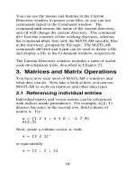
3.1 Referencing individual entries
Individual matrix and vector entries can be referenced

with indices inside parentheses. For example,
A(2,3)

denotes the entry in the second row, third column of
matrix
A
. Try:
A = [1 2 3 ; 4 5 6 ; -1 7 9]
A(2,3)
Next, create a column vector,
x
, with:
x = [3 2 1]'
or equivalently:
x = [3 ; 2 ; 1]

11
With this vector,
x(3)
denotes the third coordinate of
vector
x
, with a value of
1
. Higher dimensional arrays
are similarly indexed. An array accepts only positive
integers as indices.
An array with two or more dimensions can be indexed as
if it were a one-dimensional vector. If
A

is
m
-by-
n
, then
A(i,j)
is the same as
A(i+(j-1)*m)
. This feature is
most often used with the
find
function (see Section 5.6).
3.2 Matrix operators
The following matrix operators are available in
MATLAB:
+
addition or unary plus
-
subtraction or negation
*
multiplication
^
power
'
transpose (real) or conjugate transpose (complex)
.'
transpose (real or complex)
\
left division (backslash or
mldivide

)
/
right division (slash or
mrdivide
)
These matrix operators apply, of course, to scalars (1-by-
1 matrices) as well. If the sizes of the matrices are
incompatible for the matrix operation, an error message
will result, except in the case of scalar-matrix operations
(for addition, subtraction, division, and multiplication, in
which case each entry of the matrix is operated on by the
scalar, as in
A=A+1
). Not all scalar-matrix operations are
valid. For example,
magic(3)/pi
is valid but
pi/magic(3)
is not. Also try the commands:
A^2
A*x

12
If
x
and
y
are both column vectors, then
x'*y
is their

inner (or dot) product, and
x*y'
is their outer (or cross)
product. Try these commands:
y = [1 2 3]'
x'*y
x*y'
3.3 Matrix division (slash and
backslash)
The matrix “division” operations deserve special
comment. If
A
is an invertible square matrix and
b
is a
compatible column vector, or respectively a compatible
row vector, then
x=A\b
is the solution of
A*x=b
, and
x=b/A
is the solution of
x*A=b
. These are also called the
backslash (
\
) and slash operators (
/
); they are also

referred to as the
mldivide
and
mrdivide
functions.
If
A
is square and non-singular, then
A\b
and
b/A
are
mathematically the same as
inv(A)*b
and
b*inv(A)
,
respectively, where
inv(A)
computes the inverse of
A
.
The left and right division operators are more accurate
and efficient. In left division, if
A
is square, then it is
factorized (if necessary), and these factors are used to
solve
A*x=b
. If

A
is not square, the under- or over-
determined system is solved in the least squares sense.
Right division is defined in terms of left division by
b/A

=

(A'\b')'
. Try this:
A = [1 2 ; 3 4]
b = [4 10]'
x = A\b
The solution to
A*x=b
is the column vector
x=[2;1]
.

13
Backslash is a very powerful general-purpose method for
solving linear systems. Depending on the matrix, it
selects forward or back substitution for triangular
matrices (or permuted triangular matrices), Cholesky
factorization for symmetric matrices, LU factorization for
square matrices, or QR factorization for rectangular
matrices. It has a special solver for Hessenberg matrices.
It can also exploit sparsity, with either sparse versions of
the above list, or special-case solvers when the sparse
matrix is diagonal, tridiagonal, or banded. It selects the

best method automatically (sometimes trying one method
and then another if the first method fails). This can be
overkill if you already know what kind of matrix you
have. It can be much faster to use the
linsolve
function
described in Section 5.5.
3.4 Entry-wise operators
Matrix addition and subtraction already operate entry-
wise, but the other matrix operations do not. These other
operators (
*
,
^
,
\
, and
/
) can be made to operate entry-
wise by preceding them by a period. For example, either:
[1 2 3 4] .* [1 2 3 4]
[1 2 3 4] .^ 2
will yield
[1 4 9 16]
. Try it. This is particularly
useful when using MATLAB graphics.
Also compare
A^2
with
A.^2

.
3.5 Relational operators
The relational operators in MATLAB are:

14
<
less than
>
greater than
<=
less than or equal
>=
greater than or equal
==
equal
~=
not equal
They all operate entry-wise. Note that
=
is used in an
assignment statement whereas
==
is a relational operator.
Relational operators may be connected by logical
operators:
&
and
|
or
~

not
&&
short-circuit and
||
short-circuit or
The result of a relational operator is of type
logical
,
and is either
true
(one) or
false
(zero). Thus,
~0
is
1
,
~3
is
0
, and
4

&

5
is
1
, for example. When applied to
scalars, the result is a scalar. Try entering

3

<

5,

3

>

5,

3

==

5
, and
3

==

3
. When applied to matrices of the
same size, the result is a matrix of ones and zeros giving
the value of the expression between corresponding
entries. You can also compare elements of a matrix with
a scalar. Try:
A = [1 2 ; 3 4]
A >= 2

B = [1 3 ; 4 2]
A < B
The short-circuit operator
&&
acts just like its non-short-
circuited counterpart (
&
), except that it evaluates its left