Three-Dimensional Graphics
Bạn đang xem bản rút gọn của tài liệu. Xem và tải ngay bản đầy đủ của tài liệu tại đây (72.81 KB, 5 trang )
78
or
File
►
Save
. This saves the figure as a
.fig
file,
which can be later opened in the Figure window with the
open button
or with
File
►
Open
. Selecting
File
►
Export
Setup
or
File
►
Save
As
allows you to convert your figure to
many other formats.
13. Three-Dimensional Graphics
MATLAB’s primary commands for creating three-
dimensional graphics of numerically-defined functions
are
plot3
,
mesh
,
surf
, and
light
. Plotting of
symbolic functions is discussed in Chapter 16. The menu
options and commands for setting axes, scaling, and
placing text, labels, and legends on a graph also apply for
3-D graphs. A
zlabel
can be added. The
axis
command requires a vector of length 6 with a 3-D graph.
13.1 Curve plots
Completely analogous to
plot
in two dimensions, the
command
plot3
produces curves in three-dimensional
space. If
x
,
y
, and
z
are three vectors of the same size,
then the command
plot3(x,y,z)
produces a
perspective plot of the piecewise linear curve in three-
space passing through the points whose coordinates are
the respective elements of
x
,
y
, and
z
. These vectors are
usually defined parametrically. For example,
t = .01:.01:20*pi ;
x = cos(t) ;
79
y = sin(t) ;
z = t.^3 ;
plot3(x, y, z)
produces a helix that is compressed near the x-y plane (a
“slinky”). Try it.
13.2 Mesh and surface plots
The
mesh
command draws three-dimensional wire mesh
surface plots. The command
mesh(z)
creates a three-
dimensional perspective plot of the elements of the matrix
z
. The mesh surface is defined by the z-coordinates of
points above a rectangular grid in the x-y plane. Try
mesh(eye(20))
.
Similarly, three-dimensional faceted surface plots are
drawn with the command
surf
. Try
surf(eye(20))
.
To draw the graph of a function z = f (x, y) over a
rectangle, first define vectors
xx
and
yy
, which give
partitions of the sides of the rectangle. The function
[x,y]=meshgrid(xx,yy)
then creates a matrix
x
, each
row of which equals
xx
(whose column length is the
length of
yy
) and similarly a matrix
y
, each column of
which equals
yy
. A matrix
z
, to which
mesh
or
surf
can
be applied, is then computed by evaluating the function
f
entry-wise over the matrices
x
and
y
.
You can, for example, draw the graph of z = e
−x
2
−y
2
over
the square [-2, 2]
x
[-2, 2] as follows:
xx = -2:.2:2 ;
yy = xx ;
[x, y] = meshgrid(xx, yy) ;
z = exp(-x.^2 - y.^2) ;
mesh(z)
80
Try this plot with
surf
instead of
mesh
. Note that you
must use
x.^2
and
y.^2
instead of
x^2
and
y^2
to
ensure that the function acts entry-wise on
x
and
y
.
13.3 Parametrically defined surfaces
Plots of parametrically defined surfaces can also be made.
See the MATLAB functions
sphere
and
cylinder
for
example. The next example displays the cover of this
book, with lighting, color, and viewpoint defined in
Section 13.6. First, start a figure and set up the mesh:
figure(1) ; clf
t = linspace(0, 2*pi, 512) ;
[u,v] = meshgrid(t) ;
Next, define the surface:
2
a = -0.2 ; b = .5 ; c = .1 ;
n = 2 ;
x = (a*(1-v/(2*pi)).*(1+cos(u)) + c) ...
.* cos(n*v) ;
y = (a*(1-v/(2*pi)).*(1+cos(u)) + c) ...
.* sin(n*v) ;
z = b*v/(2*pi) + ...
a*(1-v/(2*pi)) .* sin(u) ;
Plot the surface, using
y
to define the color, and turn off
the mesh lines on the surface:
surf(x,y,z,y)
shading interp
Also try
a=-0.5
, which gives the back cover.
2
von Seggern, CRC Standard Curves and Surfaces, 2nd ed.,
CRC Press, 1993, pp. 306-307.
81
Other three-dimensional plotting functions you may wish
to explore via
help
or
doc
are
meshz
,
surfc
,
surfl
,
contour
, and
pcolor
. For plotting symbolically
defined parametric surfaces (including the same seashell
you plotted above), see Section 16.7.
13.4 Volume and vector visualization
MATLAB has an extensive suite of volume and vector
visualization tools. The following example evaluates a
function of three variables, v=f(x,y,z), that represents a
fluid flow problem. It returns both
v
and the coordinates
(
x
,
y
, and
z
) at which the function was evaluated.
[x,y,z,v] = flow ;
Now try visualizing it. The first method plots the surface
at which
v
is -3; the second plots slices of the data:
figure(1) ; clf
isosurface(x, y, z, v, -3)
figure(2) ; clf
slice(x, y, z, v, [3 8], 0, 0)
Type
doc
specgraph
for more volume and vector
visualization tools.
13.5 Color shading and color profile
The color shading of surfaces is set by the
shading
command. There are three settings for shading:
faceted
(default),
interpolated
, and
flat
. These are set by
the commands:
shading faceted
shading interp
shading flat
82
Note that on surfaces produced by
surf
, the settings
interpolated
and
flat
remove the superimposed
mesh lines. Experiment with various shadings on the
surface produced above. The command
shading
(as
well as
colormap
and
view
described below) should be
entered after the
surf
command.
The color profile of a surface is controlled by the
colormap
command. Available predefined color maps
include
hsv
(the default),
hot
,
cool
,
jet
,
pink
,
copper
,
flag
,
gray
,
bone
,
prism
, and
white
. The
command
colormap(cool)
, for example, sets a certain
color profile for the current figure. Experiment with
various color maps on the surface produced above. See
also
help
colorbar
.
13.6 Perspective of view
The Figure window provides a wide range of controls for
viewing the figure. Select
View
►
Camera
Toolbar
to
see these controls, or pull down the
Tools
menu. Try,
for example, selecting
Tools
►
Rotate
3D
, and then
click the mouse in the Figure window and drag it to rotate
the object. Some of these options can be controlled by
the
view
and
rotate3d
commands, respectively.
The MATLAB function
peaks
generates an interesting
surface on which to experiment with
shading
,
colormap
, and
view
. Type
peaks
, select
Tools
►
Rotate
3D
, and click and drag the figure to rotate it.
In MATLAB, light sources and camera position can be
set. Taking the
peaks
surface from the example above,
select
Insert
►
Light
, or type
light
to add a light