Short circuits in power systems a practical guide to IEC 60909 0 ( TQL)

Short Circuits in Power Systems


Short Circuits in Power Systems
A Practical Guide to IEC 60909-0

Ismail Kasikci

Second Edition


Author
Ismail Kasikci
Biberach University of Applied Sciences
Karlstraße 11
88400 Biberach
Germany
Cover credit Siemens

All books published by Wiley-VCH are
carefully produced. Nevertheless, authors,
editors, and publisher do not warrant the
information contained in these books,
including this book, to be free of errors.
Readers are advised to keep in mind that
statements, data, illustrations, procedural
details or other items may inadvertently
be inaccurate.
Library of Congress Card No.: applied for
British Library Cataloguing-in-Publication

Data
A catalogue record for this book is available from the British Library.
Bibliographic information published by
the Deutsche Nationalbibliothek
The Deutsche Nationalbibliothek lists
this publication in the Deutsche Nationalbibliografie; detailed bibliographic
data are available on the Internet at
.
© 2018 Wiley-VCH Verlag GmbH & Co.
KGaA, Boschstr. 12, 69469 Weinheim,
Germany
All rights reserved (including those of
translation into other languages). No part
of this book may be reproduced in any
form – by photoprinting, microfilm, or
any other means – nor transmitted or
translated into a machine language
without written permission from the
publishers. Registered names, trademarks,
etc. used in this book, even when not
specifically marked as such, are not to be
considered unprotected by law.
Print ISBN: 978-3-527-34136-8
ePDF ISBN: 978-3-527-80336-1
ePub ISBN: 978-3-527-80338-5
Mobi ISBN: 978-3-527-80339-2
oBook ISBN: 978-3-527-80337-8
Cover Design Adam-Design, Weinheim,
Germany
Typesetting SPi Global, Chennai, India

Printing and Binding
Printed on acid-free paper


v

Contents
Preface xi
Acknowledgments xiii

1.1
1.2
1.3
1.4
1.4.1
1.4.2
1.4.3
1.4.4
1.4.4.1
1.4.4.2
1.4.5
1.4.5.1
1.4.5.2
1.4.5.3
1.4.5.4
1.4.5.5
1.4.5.6

1
Time Behavior of the Short-Circuit Current 2

Short-Circuit Path in the Positive-Sequence System 3
Classification of Short-Circuit Types 5
Methods of Short-Circuit Calculation 7
Superposition Method 7
Equivalent Voltage Source 10
Transient Calculation 11
Calculating with Reference Variables 12
The Per-Unit Analysis 12
The %/MVA Method 14
Examples 14
Characteristics of the Short-Circuit Current 14
Calculation of Switching Processes 14
Calculation with pu System 14
Calculation with pu Magnitudes 16
Calculation with pu System for an Industrial System 17
Calculation with MVA System 19

2

Fault Current Analysis 23

3

The Significance of IEC 60909-0 29

4

Supply Networks 33

4.1

4.2
4.3
4.4
4.5

Calculation Variables for Supply Networks 34
Lines Supplied from a Single Source 35
Radial Networks 35
Ring Networks 35
Meshed Networks 37

1

Definitions: Methods of Calculations


vi

Contents

5

Network Types for the Calculation of Short-Circuit
Currents 39

5.1
5.2
5.3

Low-Voltage Network Types 39

Medium-Voltage Network Types 39
High-Voltage Network Types 44

6

6.6
6.6.1
6.6.1.1
6.6.1.2
6.6.2

47
TN Systems 48
Description of the System is Carried Out by Two Letters 48
Calculation of Fault Currents 49
System Power Supplied from Generators: 50
TT systems 52
Description of the System 52
IT Systems 53
Description of the System 53
Transformation of the Network Types Described to Equivalent
Circuit Diagrams 54
Examples 56
Example 1: Automatic Disconnection for a TN System 56
Calculation for a Receptacle 56
For the Heater 56
Example 2: Automatic Disconnection for a TT System 57

7

Neutral Point Treatment in Three-Phase Networks

6.1
6.1.1
6.2
6.2.1
6.3
6.3.1
6.4
6.4.1
6.5

Systems up to 1 kV

7.1
7.2
7.3
7.4
7.4.1

59
Networks with Isolated Free Neutral Point 63
Networks with Grounding Compensation 64
Networks with Low-Impedance Neutral Point Treatment 66
Examples 69
Neutral Grounding 69

8

Impedances of Three-Phase Operational Equipment 71

8.1
8.2
8.2.1
8.2.2
8.2.3
8.3
8.3.1
8.3.2
8.4
8.5
8.6
8.7
8.8
8.9
8.9.1
8.9.2

Network Feed-Ins, Primary Service Feeder 71
Synchronous Machines 73
a.c. Component 78
d.c. Component 78
Peak Value 78
Transformers 80
Short-Circuit Current on the Secondary Side 81
Voltage-Regulating Transformers 83
Cables and Overhead Lines 85
Short-Circuit Current-Limiting Choke Coils 96
Asynchronous Machines 97
Consideration of Capacitors and Nonrotating Loads 98

Static Converters 98
Wind Turbines 99
Wind Power Plant with AG 100
Wind Power Plant with a Doubly Fed Asynchronous Generator 101


Contents

8.9.3
8.10
8.11
8.11.1
8.11.2
8.11.3
8.11.4
8.11.5
8.11.6
8.11.7
8.11.7.1
8.11.7.2
8.11.7.3
8.11.7.4
8.11.7.5
8.11.7.6
8.11.7.7
8.11.7.8
8.11.7.9
8.11.7.10

Wind Power with Full Converter 101

Short-Circuit Calculation on Ship and Offshore Installations 102
Examples 104
Example 1: Calculate the Impedance 104
Example 2: Calculation of a Transformer 104
Example 3: Calculation of a Cable 105
Example 4: Calculation of a Generator 105
Example 5: Calculation of a Motor 106
Example 6: Calculation of an LV motor 106
Example 7: Design and Calculation of a Wind Farm 106
Description of the Wind Farm 106
Calculations of Impedances 111
Backup Protection and Protection Equipment 116
Thermal Stress of Cables 118
Neutral Point Connection 119
Neutral Point Transformer (NPT) 119
Network with Current-Limiting Resistor 120
Compensated Network 124
Insulated Network 125
Grounding System 125

9

Impedance Corrections 127

9.1
9.2
9.3

Correction Factor K G for Generators 128
Correction Factor K KW for Power Plant Block 129

Correction Factor K T for Transformers with Two and Three
Windings 130

10

Power System Analysis 133

10.1
10.2
10.2.1
10.3
10.4

The Method of Symmetrical Components 136
Fundamentals of Symmetrical Components 137
Derivation of the Transformation Equations 139
General Description of the Calculation Method 140
Impedances of Symmetrical Components 142

11

Calculation of Short-Circuit Currents 147

11.1
11.2
11.3
11.4
11.5
11.6
11.7

Three-Phase Short Circuits 147
Two-Phase Short Circuits with Contact to Ground 148
Two-Phase Short Circuit Without Contact to Ground 149
Single-Phase Short Circuits to Ground 150
Peak Short-Circuit Current, ip 153
Symmetrical Breaking Current, Ia 155
Steady-State Short-Circuit Current, Ik 157

12

Motors in Electrical Networks 161

12.1
12.2
12.3

Short Circuits at the Terminals of Asynchronous Motors 161
Motor Groups Supplied from Transformers with Two Windings 163
Motor Groups Supplied from Transformers with Different Nominal
Voltages 163

vii


viii

Contents

13

Mechanical and Thermal Short-Circuit Strength 167

13.1
13.2
13.3
13.4
13.4.1
13.4.2

Mechanical Short-Circuit Current Strength 167
Thermal Short-Circuit Current Strength 173
Limitation of Short-Circuit Currents 176
Examples for Thermal Stress 176
Feeder of a Transformer 176
Mechanical Short-Circuit Strength 178

14

Calculations for Short-Circuit Strength 185

14.1
14.2

Short-Circuit Strength for Medium-Voltage Switchgear 185
Short-Circuit Strength for Low-Voltage Switchgear 186

15

Equipment for Overcurrent Protection 189

16

Short-Circuit Currents in DC Systems 199

16.1
16.2
16.3
16.4
16.5

Resistances of Line Sections 201
Current Converters 202
Batteries 203
Capacitors 204
Direct Current Motors 205

17

Power Flow Analysis

17.1
17.2
17.3
17.3.1
17.3.2
17.3.3
17.3.4
17.3.5
17.3.6

17.3.6.1
17.3.6.2
17.3.7
17.3.8
17.3.9
17.3.9.1
17.3.10
17.3.11
17.3.12
17.3.13
17.3.14
17.3.14.1
17.3.14.2
17.3.14.3
17.3.14.4
17.3.14.5

207
Systems of Linear Equations 208
Determinants 209
Network Matrices 212
Admittance Matrix 212
Impedance Matrix 213
Hybrid Matrix 213
Calculation of Node Voltages and Line Currents at Predetermined
Load Currents 214
Calculation of Node Voltages at Predetermined Node Power 215
Calculation of Power Flow 215
Type of Nodes 216
Type of Loads and Complex Power 216

Linear Load Flow Equations 218
Load Flow Calculation by Newton–Raphson 219
Current Iteration 223
Jacobian Method 223
Gauss–Seidel Method 224
Newton–Raphson Method 224
Power Flow Analysis in Low-Voltage Power Systems 226
Equivalent Circuits for Power Flow Calculations 227
Examples 228
Calculation of Reactive Power 228
Application of Newton Method 228
Linear Equations 229
Application of Cramer’s Rule 229
Power Flow Calculation with NEPLAN 230


Contents

18

Examples: Calculation of Short-Circuit Currents 233

18.1
18.2
18.3
18.4
18.5
18.6
18.7
18.8

Example 1: Radial Network 233
Example 2: Proof of Protective Measures 235
Example 3: Connection Box to Service Panel 237
Example 4: Transformers in Parallel 238
Example 5: Connection of a Motor 240
Example 6: Calculation for a Load Circuit 241
Example 7: Calculation for an Industrial System 243
Example 8: Calculation of Three-Pole Short-Circuit Current and Peak
Short-Circuit Current 244
Example 9: Meshed Network 246
Example 10: Supply to a Factory 249
Example 11: Calculation with Impedance Corrections 250
Example 12: Connection of a Transformer Through an External
Network and a Generator 253
Example 13: Motors in Parallel and their Contributions to the
Short-Circuit Current 255
Example 14: Proof of the Stability of Low-Voltage Systems 257
Example 15: Proof of the Stability of Medium-Voltage and
High-Voltage Systems 259
Example 16: Calculation for Short-Circuit Currents with Impedance
Corrections 269

18.9
18.10
18.11
18.12
18.13
18.14
18.15

18.16

Bibliography 273
Standards 277
Explanations of Symbols 281
Symbols and Indices 283

Indices 286
Secondary Symbols, Upper Right, Left 287
American Cable Assembly (AWG) 287
Index 289

ix


xi

Preface
This book is the result of many years of professional activity in the area of power
supply, teaching at the VDE, as well as at the Technical Academy in Esslingen.
Every planner of electrical systems is obligated today to calculate the single-pole
or three-pole short-circuit current before and after the project management
phase. IEC 60909-0 is internationally recognized and used. This standard will
be discussed in this book on the basis of fundamental principles and technical
references, thus permitting a summary of the standard in the simplest and most
understandable way possible. The rapid development in all areas of technology is
also reflected in the improvement and elaboration of the regulations, in particular in regard to IEC 60909-0. Every system installed must not only be suitable for
normal operation, but must also be designed in consideration of fault conditions
and must remain undamaged following operation under normal conditions and
also following a fault condition. Electrical systems must therefore be designed

so that neither persons nor equipment are endangered. The dimensioning, cost
effectiveness, and safety of these systems depend to a great extent on being able
to control short-circuit currents. With increasing power of the installation, the
importance of calculating short-circuit currents has also increased accordingly.
Short-circuit current calculation is a prerequisite for the correct dimensioning of
operational electrical equipment, controlling protective measures and stability
against short circuits in the selection of equipment. Solutions to the problems
of selectivity, back-up protection, protective equipment, and voltage drops in
electrical systems will not be dealt with in this book. The reduction factors, such
as frequency, temperatures other than the normal operating temperature, type
of wiring, and the resulting current carrying capacity of conductors and cables
will also not be dealt with here.
This book comprises the following sections:
Chapter 1 describes the most important terms and definitions, together with
relevant processes and types of short circuits.
Chapter 2 is an overview of the fault current analysis.
Chapter 3 explains the significance, purpose, and creation of IEC 60909-0.
Chapter 4 deals with the network design of supply networks.
Chapter 5 gives an overview of the network types for low, medium and highvoltage network.
Chapter 6 describes the systems (network types) in the low-voltage network
(IEC 60364) with the cut-off conditions.


xii

Preface

Chapter 7 illustrates the types of neutral point treatment in three-phase networks.
Chapter 8 discusses the impedances of the three-phase operational equipment
along with relevant data, tables, diagrams, and characteristic curves.

Chapter 9 presents the impedance corrections for generators, power substation
transformers, and distribution transformers.
Chapter 10 is concerned with the power system analysis and the method of
symmetrical components. With the exception of the three-pole short-circuit current, all other fault currents are unsymmetrical. The calculation of these currents
is not possible in the positive-sequence system. The method of symmetrical components is therefore described here.
Chapter 11 is devoted to the calculation of short-circuit types.
Chapter 12 discusses the contribution of high-voltage and low-voltage motors
to the short-circuit current.
Chapter 13 deals with the subject of mechanical and thermal stresses in operational equipment as a result of short-circuit currents.
Chapter 14 gives an overview of the design values for short-circuit current
strength.
Chapter 15 is devoted to the most important overcurrent protection devices,
with time–current characteristics.
Chapter 16 gives a brief overview of the procedure for calculating short-circuit
currents in DC systems.
Chapter 17 gives an introduction into power flow analysis.
Chapter 18 represents a large number of examples taken from practice which
enhance the understanding of the theoretical foundations. A large number of
diagrams and tables that are required for the calculation simplify the application of the IEC 60909 standard as well as the calculation of short-circuit currents
and therefore shorten the time necessary to carry out the planning of electrical
systems.
I am especially indebted to Dr.-Ing. Waltraud Wüst, Dr. Martin Preuss from
Wiley-VCH and Kishore Sivakolundu from SPI for critically reviewing the
manuscript and for valuable suggestions.
At this point, I would also like to express my gratitude to all those colleagues
who supported me with their ideas, criticism, suggestions, and corrections. My
heartiest appreciation is due to Wiley Press for the excellent cooperation and their
support in the publication of this book.
Furthermore, I welcome every suggestion, criticism, and idea regarding the use
of this book from those who read the book.

Finally, without the support of my family this book could never have been written. In recognition of all the weekends and evenings I sat at the computer, I dedicate this book to my family.
Weinheim
21.07.2017

Ismail Kasikci


xiii

Acknowledgments
I would like to thank the companies Siemens and ABB for their help with figures,
pictures, and technical documentation. In particular, as a member, I am also
indebted to the VDE (Association for Electrical, Electronic and Information
Technologies) for their support and release of different kinds of tables and data.
Additionally, I would like to thank Wiley for publishing this book and especially Dr.-Ing. Waltraud Wüst, Dr. Martin Preuss from Wiley-VCH and Kishore
Sivakolundu from SPI for their assistance in supporting me and checking the
book for clarity.
Finally, I appreciate the designers and planners for their feedbacks, the students
for their useful recommendations, and the critics.


1

1
Definitions: Methods of Calculations

The following terms and definitions correspond largely to those defined in IEC
60909-0. Refer to this standard for all the terms not used in this book.
The terms short circuit and ground fault describe faults in the isolation of operational equipment, which occur when live parts are shunted out as a result.
1) Causes:

• Overtemperatures due to excessively high overcurrents;
• Disruptive discharges due to overvoltages; and
• Arcing due to moisture together with impure air, especially on insulators.
2) Effects:
• Interruption of power supply;
• Destruction of system components; and
• Development of unacceptable mechanical and thermal stresses in electrical operational equipment.
3) Short circuit: According to IEC 60909-0, a short circuit is the accidental or
intentional conductive connection through a relatively low resistance or
impedance between two or more points of a circuit that are normally at
different potentials.
4) Short-circuit current: According to IEC 60909-0, a short-circuit current
results from a short circuit in an electrical network.
It is necessary to differentiate between the short-circuit current at the position of the short circuit and the transferred short-circuit currents in the network branches.
5) Initial symmetrical short-circuit current: The effective value of the symmetrical short-circuit current at the moment at which the short circuit arises,
when the short-circuit impedance has its value from the time zero.
6) Initial symmetrical short-circuit apparent power: The short-circuit power
represents a fictitious parameter. During the planning of networks, the
short-circuit power is a suitable characteristic number.

Short Circuits in Power Systems: A Practical Guide to IEC 60909-0, Second Edition. Ismail Kasikci.
© 2018 Wiley-VCH Verlag GmbH & Co. KGaA. Published 2018 by Wiley-VCH Verlag GmbH & Co. KGaA.


2

1 Definitions: Methods of Calculations

7) Peak short-circuit current: The largest possible momentary value of the short
circuit occurring.

8) Steady-state short-circuit current: Effective value of the initial symmetrical
short-circuit current remaining after the decay of all transient phenomena.
9) Direct current (d.c.) aperiodic component: Average value of the upper and
lower envelope curve of the short-circuit current, which slowly decays
to zero.
10) Symmetrical breaking current: The effective value of the short-circuit current that flows through the contact switch at the time of the first contact
separation.
11) Equivalent voltage source: The voltage at the position of the short circuit,
which is transferred to the positive-sequence system as the only effective
voltage and is used for the calculation of the short-circuit currents.
12) Superposition method: Considers the previous load of the network before the
occurrence of the short circuit. It is necessary to know the load flow and the
setting of the transformer step switch.
13) Voltage factor: Ratio between
the equivalent voltage source and the network
√
voltage, U n , divided by 3.
14) Equivalent electrical circuit: Model for the description of the network by an
equivalent circuit.
15) Far-from-generator short circuit: The value of the symmetrical alternating
current (a.c.) periodic component remains essentially constant.
16) Near-to-generator short circuit: The value of the symmetrical a.c. periodic
component does not remain constant. The synchronous machine first delivers an initial symmetrical short-circuit current, which is more than twice the
rated current of the synchronous machine.
17) Positive-sequence short-circuit impedance: The impedance of the positivesequence system as seen from the position of the short circuit.
18) Negative-sequence short-circuit impedance: The impedance of the negativesequence system as seen from the position of the short circuit.
19) Zero-sequence short-circuit impedance: The impedance of the zero-sequence
system as seen from the position of the short circuit. Three times the value
of the neutral point to ground impedance occurs.
20) Short-circuit impedance: Impedance required for the calculation of the

short-circuit currents at the position of the short circuit.

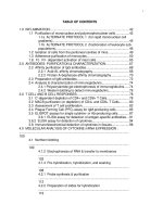
1.1 Time Behavior of the Short-Circuit Current
Figure 1.1 shows the time behavior of the short-circuit current for the occurrence
of far-from-generator and near-to-generator short circuits.
The d.c. aperiodic component depends on the point in time at which the short
circuit occurs. For a near-to-generator short circuit, the subtransient and the
transient behaviors of the synchronous machines are important. Following the
decay of all transient phenomena, the steady state sets in.


1.2 Short-Circuit Path in the Positive-Sequence System

Current
Top envelope

2√2Ik=2√2I″k

A

ip

2√2I″k

d.c. component id.c.of the short-circuit current

Time

Bottom envelope

(a)
Current

Top envelope

2√2Ik

A

ip

2√2I″k

d.c. component id.c.of the short-circuit current

Time

(b)

Bottom envelope

Figure 1.1 Time behavior of the short-circuit current (see Ref. [1]). (a) Far-from-generator short
circuit and (b) near-to-generator short circuit. Ik′′ : initial symmetrical short-circuit current; ip :
peak short-circuit current; id.c. : decaying d.c. aperiodic component; and A: initial value of d.c.
aperiodic component.

1.2 Short-Circuit Path in the Positive-Sequence System
For the same external conductor voltages, a three-phase short circuit allows
three currents of the same magnitude to develop among the three conductors.
Therefore, it is only necessary to consider one conductor in further calculations.

Depending on the distance from the position of the short circuit from the
generator, it is necessary to consider near-to-generator and far-from-generator
short circuits separately. For far-from-generator and near-to-generator short
circuits, the short-circuit path can be represented by a mesh diagram with an
a.c. voltage source, reactances X, and resistances R (Figure 1.2). Here, X and R
replace all components such as cables, conductors, transformers, generators,
and motors.

3


4

1 Definitions: Methods of Calculations

Xk

Rk

ik
~

ˆ sin ωt
u(t) = u

Figure 1.2 Equivalent circuit of the
short-circuit current path in the
positive-sequence system.

ib

R
X

The following differential equation can be used to describe the short-circuit
process:
dik
= û ⋅ sin(𝜔t + 𝜓)
(1.1)
dt
where 𝜓 is the phase angle at the point in time of the short circuit. The inhomogeneous first-order differential equation can be solved by determining the
homogeneous solution ik and a particular solution Ik′′ .
ik ⋅ Rk + Lk

ik = i′′k∼ + ik−

(1.2)

The homogeneous solution, with the time constant 𝜏 g = L/R, yields the
following:
ik = √

−û
(R2

+

X2)

et∕𝜏g sin(𝜓 − 𝜑k )

(1.3)

For the particular solution, we obtain the following:
−û
i′′k = √
sin(𝜔t + 𝜓 − 𝜑k )
(R2 + X 2 )

(1.4)

The total short-circuit current is composed of both the components:
ik = √

−û
(R2

+

X2)

[sin(𝜔t + 𝜓 − 𝜑k ) − et∕𝜏g sin(𝜓 − 𝜑k )]

(1.5)

The phase angle of the short-circuit current (short-circuit angle) is then, in
accordance with the above equation,
X
𝜑k = 𝜓 − 𝜈 = arctan
(1.6)
R

Figure 1.3 shows the switching processes of the short circuit.
For the far-from-generator short circuit, the short-circuit current is, therefore,
made up of a constant a.c. periodic component and the decaying d.c. aperiodic
component. From the simplified calculations, we can now reach the following
conclusions:
1) The short-circuit current always has a decaying d.c. aperiodic component in
addition to the stationary a.c. periodic component.
2) The magnitude of the short-circuit current depends on the operating angle of
the current. It reaches a maximum at 𝛾 = 90∘ (purely inductive load). This case
serves as the basis for further calculations.
3) The short-circuit current is always inductive.


1.3 Classification of Short-Circuit Types

ik
κ

2 I″k

id.c.

2 I″k

ikd

0

90

180

270

360

450

540

630

720

Figure 1.3 Switching processes of the short circuit.

1.3 Classification of Short-Circuit Types
For a three-phase short circuit, three voltages at the position of the short circuit
are zero. The conductors are loaded symmetrically. Therefore, it is sufficient
to calculate only in the positive-sequence system. The two-phase short-circuit
current is less than that of the three-phase short circuit, but largely close to
synchronous machines. The single-phase short-circuit current occurs most
frequently in low-voltage (LV) networks with solid grounding. The double
ground connection occurs in networks with a free neutral point or with a ground
fault neutralizer grounded system.
For the calculation of short-circuit currents, it is necessary to differentiate
between the far-from-generator and the near-to-generator cases.
1) Far-from-generator short circuit
When double the rated current is not exceeded in any machine, we speak of a
far-from-generator short circuit.

Ik′′ < 2 ⋅ IrG

(1.7)

or when
Ik′′ = Ia = Ik

(1.8)

2) Near-to-generator short circuit
When the value of the initial symmetrical short-circuit current Ik′′ exceeds
double the rated current in at least one synchronous or asynchronous machine
at the time the short circuit occurs, we speak of a near-to-generator short
circuit.
Ik′′ 2 > IrG

(1.9)

5


6

1 Definitions: Methods of Calculations

or when
Ik′′ > Ia > Ik

(1.10)

Figure 1.4 schematically illustrates the most important types of short circuits
in three-phase networks.
1) Three-phase short circuits:
• connection of all conductors with or without simultaneous contact to
ground;
• symmetrical loading of the three external conductors;
• calculation only according to single phase.
2) Two-phase short circuits:
• unsymmetrical loading;
• all voltages are nonzero;
• coupling between external conductors;
′′
′′
> Ik3
• for a near-to-generator short circuit Ik2
3) Single-phase short circuits between phase and PE:
• very frequent occurrence in LV networks.
4) Single-phase short circuits between phase and N:
• very frequent occurrence in LV networks.
5) Two-phase short circuits with ground:
• in networks with an insulated neutral point or with a suppression coil
′′
′′
< Ik2E
.
grounded system IkEE

L3

L3

L2

L2

L1

L1
I″k3

(a)

I″k2

(b)
L3

L3

L2

L2

L1

L1
I″k2EL3

I″k2EL2
I″k1

I″kE2E
(c)

(d)
Short-circuit current

Partial short-circuit currents
in conductors and earth return

Figure 1.4 Types of short-circuit currents in three-phase networks [1].


1.4 Methods of Short-Circuit Calculation

With a suppression coil grounded system, a residual ground fault current I Rest
occurs. I C and I Rest are special cases of Ik′′ .

1.4 Methods of Short-Circuit Calculation
The measurement or calculation of short-circuit current in LV networks on final
circuits is very simple. In meshed and extensive power plants, the calculation is
more difficult because of the short-circuit current of several partial short-circuit
currents in conductors and earth return.
The short-circuit currents in three-phase systems can be determined by three
different calculation procedures:
1) superposition method for a defined load flow case;
c⋅U
2) calculating with the equivalent voltage source √ n at the fault location; and
3
3) transient calculation.

1.4.1

Superposition Method

The superposition method is an exact method for the calculation of the shortcircuit currents. The method consists of three steps. The voltage ratios and
the loading condition of the network must be known before the occurrence of
the short circuit. In the first step, the currents, voltages, and internal voltages
for steady-state operation before onset of the short circuit are calculated
(Figure 1.5b). The calculation considers the impedances, power supply feeders,
and node loads of the active elements. In the second step, the voltage applied to
the fault location before the occurrence of the short circuit and the current distribution at the fault location are determined with a negative sign (Figure 1.5b).
This is the only voltage source in the network. The internal voltages are shortcircuited. In the third step, both the conditions are superimposed. We then
obtain a zero voltage at the fault location. The superposition of the currents also
leads to the value zero. The disadvantage of this method is that the steady-state
condition must be specified. The data for the network (effective and reactive
power, node voltages, and the step settings of the transformers) are often
difficult to determine. The question also arises: Which operating state leads to
the greatest short-circuit current?
The superposition method assumes that the power flow is known of the network before the fault inception and the setting of the tap changer of the transformer and the voltage set points of the generators.
By the superposition method, the power state is superimposed with an amendments state before the short circuit occurs. For this condition, the consideration
of positive sequence is sufficient.
The network consists of i = 1,…,n load nodes and j = 1,…,m generators and
power supply applications. With a suitable program, the load flow can be calculated for a network condition. After the changes in the network through the
short circuit, there are other values at each node. For a three-phase short circuit,
the voltage at the fault point equals zero. This condition is also fulfilled when the

7


Positive-sequence

1

G
3~

m

XQ

1

.
.
.

.
.
.
.
.

F

~

n

.
.

.
.
X″d .

E″
~

(b)

U(1)Q

.
.
.
.
.
.

~

~

+ U(1)f

+ U(1)f

+

.

.
X″d .

F
~

n

XQ

1

n

1
F

U(1)Q

(c)

XQ

~

E″
~

(a)

.
.
.
.
.
.

.
.
X″d .

.
.
.
.
.
.

1
F
n

~

– U(1)f

– U(1)f
(d)

Figure 1.5 Methods for the short-circuit calculation. (a) Single line diagram; (b) voltage source at the fault location; (c) superposition; and (d) equivalent

voltage source.


1.4 Methods of Short-Circuit Calculation

same voltage is given at the fault location but with an opposite voltage sign. All
network feeders, synchronous, and asynchronous machines are replaced by their
internal impedances (Figure 1.5d).
The calculation of a short-circuit current is a linear problem that can be solved
easily with linear equations. There is a linear relationship between the node voltages and node currents.
With the help of nodal admittance matrix systems, linear equations can be
solved. All impedances are converted to the LV side of the transformers. In contrast to the load flow calculation, an iteration is not required. The equations are
obtained at the short-circuit location i in matrix notation.
i=Y ⋅u
⎡ 0 ⎤ ⎡Y 11
⎢ ⎥ ⎢
⎢ 0 ⎥ ⎢Y 21
⎢⋮⎥ ⎢ ⋮
⎢ ⎥=⎢
⎢Iki′′ ⎥ ⎢ Y
⎢ ⎥ ⎢ i1
⎢⋮⎥ ⎢ ⋮
⎢ ⎥ ⎢
⎣ 0 ⎦ ⎣Y n1

(1.11)
Y 1n ⎤ ⎡ U 1 ⎤
⎥
⎥ ⎢
Y 2n ⎥ ⎢ U 2 ⎥

⎥
⎢
⋮ ⎥ ⎢ ⋮ ⎥
⎥⋅⎢ U ⎥
Y in ⎥ ⎢−c √n3 ⎥
⎥
⋮ ⎥ ⎢ ⋮ ⎥
⎥
⎥ ⎢
Y nn ⎦ ⎢ U ⎥
⎣ n ⎦

(1.12)

After inversion, we obtain the following:
u = Y −1 ⋅ i
⎡ U 1 ⎤ ⎡Z
11
⎢
⎥
⎢ U 2 ⎥ ⎢⎢Z21
⎢
⎥
⎢ ⋮ ⎥ ⎢⎢ ⋮
Un ⎥ =
⎢−c √
⎢Z
⎢
i1
3⎥

⎢
⎥ ⎢⎢ ⋮
⋮
⎢
⎥
⎢ U ⎥ ⎢⎣Z
n1
⎣ n ⎦

(1.13)
Z1n ⎤ ⎡ 0 ⎤
⎥ ⎢ ⎥
Z2n ⎥ ⎢ 0 ⎥
⋮ ⎥ ⎢⋮⎥
⎥⋅⎢ ⎥
Zin ⎥ ⎢Iki′′ ⎥
⎥ ⎢ ⎥
⋮ ⎥ ⎢⋮⎥
⎥ ⎢ ⎥
Znn ⎦ ⎣0n ⎦

(1.14)

From the ith row of the equation results
U
−c √n = Z ii ⋅ I ′′ki
3

(1.15)

The initial short-circuit a.c. can be calculated by redirecting the above equation:
c⋅U
I ′′ki = − √ n
3 ⋅ Zii

(1.16)

For the node voltages, follow:
U k = Zki ⋅ I ′′ki

(1.16a)

9


10

1 Definitions: Methods of Calculations

Since the operating voltage U(1)f = √Un3 is not known at the fault location, for the
equivalent voltage source at the fault point can be introduced.
c⋅U
−U (1)f = √ n
(1.17)
3
At the short-circuit point, the only active voltage is the Thevenin equivalent
voltage source of the system.
1.4.2

Equivalent Voltage Source

Figure 1.6 shows an example of the equivalent voltage source at the short-circuit
location F as the only active voltage of the system fed by a transformer with
or without an on-load tap changer. All other active voltages in the system
are short-circuited. Thus, the network feeder is represented by its internal
impedance, ZQt , transferred to the LV side of the transformer and the transformer by its impedance referred to the LV side. The shunt admittances of the line,
the transformer, and the nonrotating loads are not considered. The impedances
of the network feeder and the transformer are converted to the LV side.
The transformer is corrected with K T , which will be explained later.
The voltage factor c (Table 1.1) will be described briefly as follows:
If there are no national standards, it seems adequate to choose a voltage factor c, according to Table 1.1, considering that the highest voltage in a normal
Q

HV

T

LV

A

t:1

UnQ

F

Cable line

Fault location

Load
P, Q

I″kQ

Load
P, Q

(a)
RQ
UqQ

jXQ

Q

RT

jXT

A

RL

jXL

F

UQ

I″k

3
01
RQt

jXQt Q

RTLVK jXTLVK A

RL

F

jXL

c.Un
01

I″k

3

(b)

Figure 1.6 Network circuit with equivalent voltage source [2]. (a) System diagram and
(b) equivalent circuit diagram of the positive-sequence system.

1.4 Methods of Short-Circuit Calculation

Table 1.1 Voltage factor c, according to IEC 60909-0: 2016-10 [1].
Nominal voltage, Un

Voltage factor c for calculation of
Maximum short-circuit
currents (cmax )a)

Minimum short-circuit
currents (cmin )

Low voltage
100–1000 V

1.05b)

0.95b)

(IEC 38, Table I)

1.10c)

0.9c)

1.10

1.00

High voltaged)

>1–35 kV
(IEC 38, Tables III and IV)
a) cmax U n should not exceed the highest voltage U m for equipment of power systems.
b) For LV systems with a tolerance of ±6%, for example, systems renamed from 380 to
400 V.
c) For LV systems with a tolerance of ±10%.
d) If no nominal voltage is defined, cmax U n = U m or cmin U n = 0.90 U m should be applied.

(undisturbed) system does not differ, on average, by more than approximately
+5% (some LV systems) or +10% (some high-voltage, HV, systems) from the nominal system voltage U n [3].
1) The different voltage values depending on time and position
2) The step changes of the transformer switch
3) The loads and capacitances in the calculation of the equivalent voltage source
can be neglected
4) The subtransient behavior of generators and motors must be considered.
This method assumes the following conditions:
1)
2)
3)
4)

The passive loads and conductor capacitances can be neglected
The step setting of the transformers need not be considered
The excitation of the generators need not be considered
The time and position dependence of the previous load (loading state) of the
network need not be considered.

1.4.3

Transient Calculation

With the transient method, the individual operating equipment and, as a result,
the entire network are represented by a system of differential equations. The
calculation is very tedious. The method with the equivalent voltage source is a
simplification relative to the other methods. Since 1988, it has been standardized internationally in IEC 60909-0. The calculation is independent of a current
operational state. Therefore, in this book, the method with the equivalent voltage
source will be dealt with and discussed.

11


12

1 Definitions: Methods of Calculations

1.4.4

Calculating with Reference Variables

There are several methods for performing short-circuit calculations with absolute and reference impedance values. A few methods are summarized here, and
examples are calculated for comparison. To define the relative values, there are
two possible reference variables.
For the characterization of electrotechnical relationships, we require the four
parameters:
1)
2)
3)
4)

voltage U in V;

current I in A;
impedance Z in Ω; and
apparent power S in VA.
Three methods can be used to calculate the short-circuit current:

1) The Ohm system: units – kV, kA, V, and MVA.
2) The per-unit (pu) system: this method is used predominantly for electrical
machines; all four parameters u, i, z, and s are given as per unit (unit = 1). The
reference value is 100 MVA. The two reference variables for this system are
U B and SB . Example: The reactances of a synchronous machine X d , Xd′ , and
Xd′′ are given in pu or in %pu, multiplied by 100%.
3) The %/MVA system: this system is especially well suited for the quick determination of short-circuit impedances. As a formal unit, only the % symbol is
added.
1.4.4.1

The Per-Unit Analysis

Today, the power system consists of complex and complicated mesh, ring, and
radial networks with many transformers, generators, and cables. The calculation of such a circuit can be very tedious and incorrect. The use of sophisticated
computer programs is a big help for engineers. On the other hand, for a quick
calculation a simple method, per unit system also can be used. However, this
method is not accepted worldwide and is not standardized by IEC, EN, or IEEE
committees.
The pu method uses the electrical variables U, I, Z, and S. They are based on a
dimensionless same references, namely, U base , I base , Zbase , or Sbase . The resulting
dimensionless quantities are described with the lowercase u, i, z, or s.
A pu system is defined as follows:
the actual value (in any unit)
Per unit value (pu) =
the base or reference value (in the same unit)

U
upu =
Ubase
A reference voltage and a reference apparent power are selected and then reference current and impedance are calculated as follows:
U2
Zbase = base
Sbase
Sbase
Ibase =
Ubase


1.4 Methods of Short-Circuit Calculation

Only a single global base value is selected in the short-circuit current
calculation. This reference value is then used for all other networks. The choice
of reference values can be carried out arbitrarily in principle. However, it is
appropriate to select the rated voltage at the short-circuit location as a reference
voltage. For example, as reference apparent power is the rated apparent power
of the largest transformer in the network or a power of the same selected
magnitude (e.g., 100 MVA). The best choice of base can be achieved when the
impedances and currents in easily handled orders of magnitude.
It should be noted that related parameters’ individual resources, such as the relative short-circuit voltage of a transformer ukr or related subtransient reactance
x′′d of the generator, are always relative to a base, which consists of the design
parameters of the particular equipment. In a short-circuit current calculation as
per pu method, these parameters must first be converted to the selected global
basis. If we give an example for voltage and current, the expression is as follows:
U
Upu = actual
Ubase

Iactual
Ipu =
Ibase
Note that the voltage according to the international system of units (SI) is not
V , but U. The letter V is a unit in this case. V is used especially in Anglo-Saxon
countries.
For other values, we can write for 1 pu impedance (Ω):
Upu
U
U
Zbase = base = base or in pu Zpu =
Ibase
Ibase
Ipu
Sbase
Ibase =
Ubase
We convert the values to pu:
R
Rpu =
Zbase
X
Xpu =
Zbase
Remember that a symmetrical three-phase system has two voltages, line–line
voltage U L (U n ) and U LN (U 0 ). By definition:
U
ULN = √L
3
Now consider:

ULN
ULNpu =
ULNbase
It follows that:
√
ULN
UL ∕ 3
UL
=
= ULpu
ULNpu =
√ =
ULNbase
U
Lbase
ULbase ∕ 3
√
Consider that the factor 3 disappears in the pu equation.

13