Dynamic instability of thin plates by the dynamic stiffness method
Bạn đang xem bản rút gọn của tài liệu. Xem và tải ngay bản đầy đủ của tài liệu tại đây (460.51 KB, 11 trang )
Thông báo Khoa học và Công nghệ* Số 1-2013
54
DYNAMIC INSTABILITY OF THIN PLATES BY THE DYNAMIC
STIFFNESS METHOD
Master Hung Quoc Huynh
Faculty of Civil Engineering, Central University of Construction
Abtract: Dynamic instability of thin rectangular plates subjected to uniform in-plane
harmonic compressive load applied alon
g two opposite edges are investigated in this paper. The dynamic stiffness method (DSM), as
a consequence the dynamic stiffness matrices, is used to analyze the free vibration, the static
stability, and dynamic instability of thin plates under different boundary conditions. The
boundaries of the dynamic instability principal regions are obtained using Bolotin’s
method. Results obtained such as free vibration frequencies, static buckling critical load
and dynamic instability principal regions are compared with the results previously
published to ascertain the validity of the method.
Keywords: Dynamic stability; static stability; dynamic stiffness method; plate
1. Introduction
Various plate structures are widely used in
aircraft, ship, bridge, building, and some
other engineering activities. In many
circumstances, these structures are exposed
to dynamic loading. Plate structures are often
designed to withstand a considerable in-plane
load along with the transverse loads. The
dynamic instability of thin rectangular plates
under periodic in-plane loads has been
investigated by a number of researchers.
The dynamic stability of rectangular plates
under various in-plane periodic forces was
studied by Bolotin [1], as well as by Yamaki
and Nagai [2]. Hutt and Salama [3]
demonstrated the application of the finite
element method to the dynamic stability of
plates subjected to uniform harmonic loads.
Takahasi and Konishi [4] studied the
dynamic stability of a rectangular plate
subjected to a linearly distributed load such
as pure bending or a triangularly distributed
load applied along the two opposite edges
using harmonic balance method. Nguyen and
Ostiguy [5] considered the influence of the
aspect ratio and boundary conditions on the
dynamic instability and non-linear response
of rectangular plates. Guan-Yuan Wu and
Yan-shin Shih [6] investigated the effects of
various system parameters on the regions of
instability and the non-linear response
characteristics of rectangular cracked plates
using incremental harmonic balance (IHB)
method. The dynamic instability behaviour
of rectangular plates under periodic in-plane
normal and shear loadings was studied by
Singh and Dey [7] using energy-based finite
difference method. Srivastava et al. [8]
employed the nine-noded isoparametric
quadratic element with five degree-offreedom method to investigate the dynamic
instability of stiffened plates subjected to
non-uniform harmonic in-plane edge loading.
Thông báo Khoa học và Công nghệ* Số 1-2013
In this paper, the problem of dynamic
stability of plates subjected to periodic inplate load along two opposite edges is
studied by the dynamic stiffness method. The
problem is solved by the dynamic stiffness
method in order to investigate the efficiency
and the reliability of this method for solving
above-mentioned problems. The boundaries
of the dynamic instability principal regions
are obtained using Bolotin’s method. The
dynamic stability equation is solved to plot
the relationship of the parameters of load,
natural frequency, frequency of excitation
from the computational program by Matlab.
Results obtained, such as free vibration
frequencies, static buckling critical load, and
principal regions of dynamic instability, are
compared with the results previously
published to ascertain the validity of the
method.
2. Dynamic stability analysis
Assume that a rectangular plate with
length a, width b, and thickness h is
subjected to uniform harmonic in-plane loads
Nx applied along the two opposite
boundaries. Both unloaded edges can be
simply supported (SS) or clamped (C). A
Cartesian co-ordinate system (x, y, z) is
introduced as shown in Fig. 1.
Nx = Ns + Nt cos t
Nx
x, u
lf-w
ave
O
y v
h
a
in o
ne
ling
Edge b
b
Bu
ck
SS
z,w
ha
Edge a
SS
The dynamic instability analysis of
composite laminated rectangular plates and
prismatic plate structures was determined by
Wang and Dawe [9] using the finite strip
method. Wu Lanhe et al. [10] analyzed the
dynamic stability of thick functionally graded
material plates subjected to aero-thermomechanical loads, using a novel numerical
solution technique, the moving least squares
differential quadrature method. The dynamic
instability of laminated sandwich plates
subjected to in-plane edge loading was
studied by Anupam Chakrabarti and Abdul
Hamid Sheikh [11] using the proposed finite
element plate model based on refined higher
order shear deformation theory. Dynamic
stability analysis of composite plates
including delaminations were performed by
Adrian G. Radu and Aditi Chattopadhyay
[12] using a higher order theory and
transformation matrix approach.
55
Buckling in several half-waves
Fig. 1. Rectangular plate subjected to
dynamic inplane loads.
The equations of motion for generally
isotropic plates are given by Timoshenko
[13], and can be reduced to the following set
of equations
2w
2w
N
0
x
t2
x2
(1)
4w
4w 4w
w 4 2 2 2 4
x
x y y
(2)
D4w h
in which
4
where w is the displacement at mid-surface in
z-direction
of
rectangular
Cartesian
Thông báo Khoa học và Công nghệ* Số 1-2013
coordinates, t is the time, and is the mass
density per unit volume. The flexural rigidity
is defined as D = Eh3/12(1-2 ) in which E is
Young’s modulus and is Poisson ratio.
In the above equation, the in-plane load
factor Nx is periodic and can be expressed in
the form:
Nx Ns Nt cosΩt
(3)
where Ns is the static portion of Nx, Nt is the
amplitude of the dynamic portion of Nx, and
is the frequency of excitation. The lowest
critical static buckling load Ncr may be
expressed interns of Ns and Nt as follows:
(4)
N s s N cr , N t d N cr
where s and d are static and dynamic load
factors, respectively.
The transverse deflection function w,
satisfying the geometric boundary conditions,
can be written as
N
w( x, y, t ) Ym ( y )sin
m 1
m x
f (t )
a
(5)
where m is the number of half-waves (normal
spatial mode in x-direction), a is the length of
plate in x-direction, f(t) are unknown
functions of time, and Ym(y) are functions to
be determined in order to satisfy the equation
of motion (1).
By substituting Eq. (5) into Eq. (1), the
following fourth order ordinary differential
equations are obtained
h
Ym f (t ) YmIV 2 k m2 Ym'' k m4 Ym
D
( N d N cr cosΩt ) 2
s cr
k m Ym f (t ) 0
D
where
km m / a
(6)
(7)
Equations (6) represent a system of secondorder differential equations for the time
56
functions with periodic coefficients of the
standard Mathieu-Hill equations, describing
the instability behavior of the plate subjected
to a periodic in-plane compressive load.
The analysis of a given structural system
for
dynamic
stability
implies
the
determination of boundaries between the
stable and unstable regions. The dynamic
instability boundaries are determined using
the method suggested by Bolotin [1]. The
stability and instability of their solution
depends on the parameters of the system. The
boundaries between stable and unstable
regions in the parameter space are formed by
periodic solutions of period T and 2T, where
T = 2/. The principal instability region
(first instability region) is usually the most
important in dynamic stability analysis,
because of its width as well as due to
structural damping, which often neutralize
higher regions.
The boundaries of the principal instability
region with period of 2T are of practical
importance and their solution can be
achieved in the form of Fourier series
f (t )
k t
k t
bk cos
ak sin
2
2
k 1,3,5,...
(8)
where ak and bk are vectors independent of
time.
Substitution of equations (8) into
equations (6) leads to an eigenvalue system
for the dynamic stability boundary
1 4 0
4 2 4 0
0 4 3 4
0
(9)
Thông báo Khoa học và Công nghệ* Số 1-2013
where
1 YmIV
3.1. Generalized displacements
2km2 Ym''
YmIV
Mym2 Q ym2
a
y, v
h
Wm2
Fig. 2. Generalized displacements
generalized forces of plate.
25Ω 2 h s N cr 2
km4
km Ym
4 D
D
and
Generalized displacement vector can be
expressed as
d Ncr 2
kmYm
2 D
It has been shown by Bolotin [l] that
solutions with period 2T are the ones of
greatest practical importance, and that as a
first approximation the boundaries of the
principal regions of dynamic instability can
be determined from element (1, 1) of
determinant (9)
YmIV 2km2 Ym''
2
(10)
km4 Ω h ( s 1 d ) N cr km2 Ym 0
4 D
2
D
3. Dynamic stiffness method
uT Wm1 ( x,0)
Wm' 1 ( x,0)
Wm 2 ( x, b)
Wm' 2 ( x, b)
(13)
then
Wm1 ( x,0) Ym (0); Wm' 1 ( x,0) Ym' (0);
Wm 2 ( x, b) Ym (b ); Wm' 2 ( x, b ) Ym' (b)
(14)
The generalized displacement vector {u} can
be determined by substituting Eqs (14) into
Eqs (13) taking into account (11) and
evaluating it at y=0 and y=b, then Eq. (13)
can be rewritten in matrix form
(15)
u K1 C
where CT C1 C2 C3 C4 and
The general solution of differential equations
(10) has the form
(11)
where
1/2
2
c k 2 h Ω ( 1 ) N cr k 2
m
s
d
m
2
D
D 4
1/2
2
N
d k m2 h Ω ( s 1 d ) cr km2
2
D
D 4
b
'
Wm2
3 YmIV 2km2 Ym''
C3 sin( d . y ) C4 cos( d . y)
Nx
z, w
2km2 Ym''
Ym ( y ) C1sinh(c. y ) C 2cosh (c. y )
x, u
'
Wm1
Wm1
9Ω 2 h s N cr 2
km4
km Ym
4 D
D
4
Mym1 Q ym1
O
Nx
2
km4 Ω h ( s 1 d ) Ncr km2 Ym
4 D
2
D
2
57
(12)
where C1, C2, C3 and C4 are the coefficients
to be determined from the four boundary
conditions, edge a at y = 0, and edge b at y = b.
0
1
0
1
c
0
d
0
K1
sinh(bc
. ) cosh(bc
. ) sin(bd
. )
cos(bd
. )
.
(bc
. ) c.sinh(bc
. ) d.cos(bd
. ) d.sin(bd
. )
ccosh
(16)
where [K1] is the shape function.
3.2. Generalized forces
Generalized force vector can be expressed as
QT
Qym1 ( x,0)
M ym1 ( x,0)
Qym 2 ( x, b )
M ym 2 ( x, b )
(17)
The Kirchhoff shear force Qy(x,y) and the
bending moment My(x,y) of the plate along
the line y=constant are [15]
Thông báo Khoa học và Công nghệ* Số 1-2013
3 w 3 w
Qy ( x, y ) D 3 2
x y
y
2w
2w
M y ( x, y ) D 2 2
x
y
(18)
The generalized force which are determined
to Eqs (18) can be written
Qymi ( x, y ) D Y k Y
''
2
M ymi ( x, y ) D Ym kmYm
'''
m
2 '
m m
(19)
The generalized force vector {Q} can be
determined by substituting Eqs (19) into Eq.
(17) taking into account (11) and evaluating
it at y=0 and y=b, then Eq. (17) can be
rewritten in matrix form
(20)
Q K 2 C
where K 2 is the generalized stiffness matrix
k11 k12
k
k
K 2 D k21 k22
31
32
k
k
41 42
k13
k23
k33
k43
k14
k24
k34
k44
(21)
Explicit expressions of the elements kij of
the generalized stiffness matrix [K2 ] are as
follows:
58
By substituting Eq. (15) into Eq. (20), the
generalized nodal displacements and nodal
forces are related,
Q K 2 K1 1 u
Therefore, Q D u
(23)
Where
D K 2 K1 1
(24)
Matrix [D] in equation (24) is the required
dynamic stiffness matrix. With the dynamic
stiffness matrix being available, the
vibration, static stability and dynamic
stability problems of the plate structures can
be solved.
3.3. Static stability and vibration of the plate
Two parameters c and d of the dynamic
stiffness matrix [D] for solving the static
stability and vibration problem are
determined as follows :
4
2
c k 2 2 r k 2
m
m m m
a
a
4
2
r
d km2 m2 km2 m
a
a
(25)
k11 (c.km2 c3 );
k12 0
where r a / b is aspect ratio of plate, N m
3
k14 0
represents the static critical load of plate for
the m mode, and m represents the non-
2
k13 (d d .km );
3
k31 (c
.cosh(bc
. ) c.km2.cosh(bc
. ))
k32 (c3.sinh(bc
. ) c.km2.sinh(bc
. ))
k33 (d3.cos(bd
. ) d.km2.cos(bd
. ))
k34 (d3.sin(bd
. ) d.km2.sin(bd
. ))
k21 0;
k22 (km2.v c2)
k23 0;
k24 (d2 vk
. m2)
k41 (c2 .sinh(b.c) km2 .v.sinh(b.c))
k42 (c2 .cosh(b.c) km2 .v.cosh(b.c))
k43 (d 2 .sin(b.d ) km2 .v.sin(b.d ))
2
2
k44 (d .cos(b.d ) km .v.cos(b.d ))
(22)
dimensional static critical loading factor of
plate for the m mode, which is defined as
m N m b2 / 2 D
(26)
The non-dimensional natural frequency
parameter (natural frequency factor) m of
plate is defined as
m m a 2 / 2
h / D
(27)
where m is the natural frequency for the m
mode of plate.
Thông báo Khoa học và Công nghệ* Số 1-2013
59
Step 4. Solve dynamic stability equation
load
* d / 2(1 s )
parameter
is
(29)
The natural frequency of lateral free
vibration of a rectangular plate loaded by a
uniform in-plane force is defined as
(30)
m* m 1 s
(34)
4. Numerical results and discussions
4.1. Static stability and vibration problems
4.1.1. Problem 1. An example is investigated
for the static stability and natural vibration
analysis of a thin square plate P1 (a=b) with
all four edges simply supported and
compressed by uniformly distributed inplane forces along its opposite edges (Fig. 3).
Nx
Nx
(a)
P.1
The non-dimensional frequency of excitation
parameter is as follows
Λ Ωa2 h / D
a=b
y
(b)
3.5. Dynamic instability of thin plates by the
dynamic stiffness method
Q D u
*
*
*
(33)
Step 3. Derive the dynamic stability equation.
For any displacemant {u *} to become
infinitely large, [D*] must vanish and this
condition
means
that
every
other
displacemant in the plate must also tend to
infinity. Therefore, for dynamic instability
the condition is det D* 0 .
Nx
Nx
Buckling in one half-wave (m = 1)
Fig. 3. Thin square plate P1 (SS-SS-SS-SS).
The dynamic stability equation (34) is
solved by plotting the relationship m-m
using Matlab program, which determines the
static critical loading factors m and the free
vibration frequency factors m.
Static critical loading factor
Step 2. Apply the constraints as dictated by
the boundary conditions. Apply boundary
conditions of the problem to eliminate
degeneracy of the dynamic stiffness matrix.
Equation (32) has the form:
b
SS
(31)
Step 1. The motion equation (23) of plate
would be:
(32)
Q Du
x
SS
Buckling in one half-wave
The normalized
determined as
det D* 0
SS
For analyzing the dynamic stability, two
parameters c and d of the dynamic stiffness
matrix [D] are determined as in Eq. (12).
The non-dimensional static critical loading
factor cr of plate is defined as
(28)
cr N cr b 2 / 2 D
SS
3.4. Dynamic instability of the plate
8
6
4
4
2
0
2
0
1
2
3
4
Natural frequency factor
5
6
Fig. 4. Relation m-m (plate P1, mode m=1).
8
Results obtained in the present analysis are
compared with those of Yamaki and Nagai
[2] and Timoshenko [13,14] in Table 1,
which shows a good agreement.
6.2499
6
4
2
0
5
0
1
2
3
4
Natural frequency factor
5
6
Fig. 5. Relation m-m (plate P1, mode m=2).
Static critical loading factor
60
12
10 11.111
8
6
4.1.2. Problem 2. This problem considers a
thin square plate P3 (a=b) with two edges
simply supported and two edges clamped
and compressed by uniformly distributed inplane forces along its opposite edges for the
static stability and free vibration frequency
(Fig. 7).
4
Nx
2
0
2
4
6
8
Natural frequency factor
x
C
10
0
10
12
Nx
(a)
SS
P.3
Fig. 6. Relation m-m (plate P1, mode m=3).
b
SS
C
It is observed from Fig. 4-6 that the lowest
static critical loading factor and the free
vibration frequency factors are determined
a=b
y
Nx
Nx
(b)
cr 4 , 1 2; 2 5; 3 10
)
The lowest static critical buckling load
Fig. 7. Thin square plate P3 (SS-C-SS-C).
10
Static critical loading factor
N cr 4 2 D / b2
The free vibration frequencies
1 2( 2 / a 2 ) D / h ;
2 5( 2 / a 2 ) D / h ;
mode
m
1
1
2
3
DSM
Ref. [2]
4
2
5
10
4
2
5
10
6
4
2
Ref.
[13,14]
4
2
5
10
2.9332
0
1
2
3
4
5
6
Natural frequency factor
7
8
9
10
Fig. 8. Relation m-m (plate P3, mode m=1).
10
Static critical loading factor
Table 1. Comparison of cr and m of square
plate P1.
factor
8.6044
8
0
3 10( 2 / a 2 ) D / h
cr
m
Buckling in one half-wave
Static critical loading factor
Thông báo Khoa học và Công nghệ* Số 1-2013
8
7.6913
6
4
2
0
5.5466
0
1
2
3
4
5
6
Natural frequency factor
7
8
9
10
Fig. 9. Relation m-m (plate P3, mode m=2).
Thông báo Khoa học và Công nghệ* Số 1-2013
12
4.2. Dynamic instability problems
11.9178
10
8
6
4
2
10.3566
0
0
2
4
6
8
10
Natural frequency factor
12
14
16
4.2.1. Problem 1. This problem concerns the
dynamic stability of a thin square plate P1
(a=b) with all four edges simply supported
and compressed by uniformly distributed inplane periodic forces along its opposite edges
(Fig. 11).
Nx = sNcr + dNcr cos t
Fig. 10. Relation m-m (plate P3, mode m=3).
SS
Nx
The lowest static critical loading
N cr 7.6913 2 D / b 2
The free vibration frequency
1 2.9332( 2 / a 2 ) D / h ;
2 5.5466( 2 / a 2 ) D / h ;
3 10.3566( 2 / a 2 ) D / h
Table 2. Comparison of cr and m of square
plate P3
P.1
b
SS
a=b
cr 7.6913 ; 1 2.9332 ; 2 5.5466 ;
3 10.3566
x
SS
It is observed from Fig. 7-10 that the lowest
static critical buckling load factor and the
free vibration frequency factors are
determined
SS
Static critical loading factor
14
61
y
Fig. 11. Thin square plate P1 (SS-SS-SS-SS).
By solving the dynamic stability Eq. (34),
we obtain the boundaries of the principal
dynamic instability regions, which are
presented in the non-dimensional frequency
of excitation parameter () versus dynamic
load factor (d) amplitude plane. Two values
of the static load factor s , i.e., 0 and 0.6, are
considered.
Case 1: the static load factor S = 0
Results obtained in the present analysis are
compared with those of Yamaki and Nagai
[2] and Timoshenko [15] in Table 2, which
shows a good agreement.
1
Unstable
0.8
s
Ref.
DSM
Ref. [2]
[15]
7.6913 7.701
7.69
2.9332 2.935
5.5466 5.550
10.3566 10.36
-
Dynamic load factor: d
1.2
mode
factor
m
2
cr
1
m
2
3
0.6
0.4
0.2
0
0
10
20
30
40
50
Dimensionless excitation frequency:
60
Fig. 12. Principal instability region for the
square plate P1 (case 1, S = 0).
Case 2: the static load factor S = 0.6
Thông báo Khoa học và Công nghệ* Số 1-2013
0.5
Unstable
0.4
Fig. 13. Principal instability region for the
square plate P1 (case 2, S = 0.6).
s
Dynamic load factor: d
Principal region of dynamic instability for simply supported plate P.1
0.6
62
0.3
0.2
0.1
0
0
10
20
30
40
50
Dimensionless excitation frequency:
60
Table 3. Comparison of principal region of dynamic instability for square plate P1 (case 1, S =
0).
d
0
0.2
0.4
0.8
1.2
Dimensionless excitation frequency
DSM
Ref. [3]
right
left
right
left
39.478
39.478
39.46
39.46
41.405
37.452
43.246
35.311
43.00
35.32
46.711
30.579
46.56
30.78
49.936
24.968
49.52
25.06
Ref. [8]
right
39.46
43.16
46.54
49.54
Ref. [11]
right
41.384
43.224
49.911
left
39.46
35.37
30.73
24.02
left
37.433
35.292
24.956
Table 4. Comparison of principal region of dynamic instability for square plate P1 (case 2, S =
0.6).
d
0
0.16
0.32
0.48
Dimensionless excitation frequency
DSM
Ref. [3]
right
left
right
24.968
24.968
25.06
27.351
22.332
27.43
29.542
19.340
29.60
31.582
15.791
31.57
Results obtained in the present analysis are
compared with those of Hutt and Salam [3],
Srivastava, Datta and Sheikh [8], and
Chakrabarti and Sheikh [11] in Table 3 and
Table 4, which show a good agreement.
Ref. [8]
right
25.04
27.41
29.58
31.55
left
25.06
22.49
19.53
15.91
left
25.04
22.48
19.51
15.89
uniformly distributed in-plane periodic forces
along its opposite edges (Fig. 14).
Nx = sNcr + dNcr cos t
x
C
Nx
4.2.2. Problem 2. An example is investigated
for the dynamic stability of a thin rectangular
plate P4 with two edges simply supported
and two edges clamped and compressed by
SS
P.4
C
a = 1.667b
y
SS
b
Thông báo Khoa học và Công nghệ* Số 1-2013
Fig. 14. Thin rectangular plate P4 (SS-C-SSC).
(mode1,2,3)
m=2
0.3
basis, the dynamic stability equation is
established to analyze the problem of static
stability, vibration and dynamic stability of
thin plates by the dynamic stiffness method.
m=3
0.2
0.1
0
0
m=1
0.5
1.5
1
Normalized frequency parameter:
2
*
Dynamic load factor: d
0.4
63
2.5
Fig.15.Principal instability regions for the
rectangular plate P4(modes m=1,2,3) for S = 0.5.
Research results obtained such as free
vibration frequencies, static critical buckling
load and principal regions of dynamic
instability for the plates by the dynamic
stiffness method are compared with the
results previously published to be in a good
agreement. Thus in the analysis of plates
structural one can use the dynamic stiffness
method as a reliable and efficient tool.
References
Fig. 16. Principal instability regions for the
rectangular plate P4 (mode m=1,2,3) for S =
0.5 of Ref. [5].
The plots of the principal region of dynamic
instability for the rectangular plate P4 for
three modes (m=1,2,3) in Fig. 15 are
compared and found to be in a very good
agreement with the results of Nguyen and
Ostiguy [5] in Fig. 16.
5. Conclussion
In the paper, the dynamic stiffness method
has been developed to analyze the thin plates
and to consider the effect of in-plane
dynamic forces on static stability, vibration
and dynamic stability of such plates.
The dynamic stiffness matrices of thin
plates subjected to uniformly distributed
static in-plane edge loading and dynamic inplane edge loading are established. On that
[1] Bolotin V.V. 1964. The dynamic stability
of elastic system, San Francisco, Holden-Day.
[2] Yamaki N., Nagai K.1975. Dynamic
stability of rectangular plates under periodic
compressive forces, Report No. 288 of the
Institute of high speed mechanics, Tohoku
University 32 103-127.
[3] Hutt J.M., Salam A.E. 1971. Dynamic
instability of plates by finite element method,
ASCE J. of Eng. Mech. 3 879-899.
[4] Takahashi K., Konishi Y. 1988. Dynamic
stability of a rectangular plate subjected to
distributed in-plane dynamic force, J. of
Sound Vib. 123 115-127.
[5] Nguyen H., Ostiguy G.L. 1989. Effect of
boundary conditions on the dynamic
instability and
non-linear response of
rectangular plates, part I, theory, J. of Sound
and Vib. 133 381-400.
[6] Guan-Yuan W., Shih Y.S. 2005 Dynamic
instability of rectangular plate with an edge
crack, Comput. and Struct. 84 1 -10.
Thông báo Khoa học và Công nghệ* Số 1-2013
[7] Singh J.P., Dey S.S. 1992. Parametric
instability of rectangular plates by the energy
based finite difference method, Comput.
Methods in Appl. Mech. and Eng. 97 1 – 21,
North-Holland.
[8] Srivastava A.K.L. 2003. Datta
P.K.,Sheikh A.H., Dynamic instability of
stiffened plates subjected to non-uniform
harmonic in-plane edge loading, J. of Sound
and Vib. 262 1171-1189.
[9] Wang S., Dawe D.J. 2002. Dynamic
instability
of
composite
laminated
rectangular plates and prismatic plate
structures, Comput. methods appl. Mech.
and eng. 191 1791–1826.
[10] Wu Lanhe, Wang Hongjun, Wang
Daobin. 2007. Dynamic stability analysis of
FGM plates by the moving least squares
differential quadrature method, Composite
Struct. 77 383–394.
64
[11] Chakrabarti A, Sheikh A.H. 2006.
Dynamic instability of laminated sandwich
plates using an efficient finite element model,
Thin-Walled Struct. 44 57-68.
[12] Adrian G., Radu, Aditi Chattopadhyay.
2002. Dynamic stability analysis of
composite plates including delaminations
using a higher order theory and
transformation matrix approach, International
J. of Solids and Struct. 39 1949-1965.
[13] Timoshenko S.P., Gere J.M. 1961
Theory of elastic stability. Tokyo: McGrawhill, Kogakusha.
[14] Timoshenko S.P., Young D.H. 1955.
Vibration Problems in Engineering, D.Van
Nostrand Co.,
[15] M.L. Gambhir. 2004. Stability analysis
and design of structures, Springer
Bất ổn định động tấm mỏng bằng phương pháp độ cứng động lực
ThS. Huỳnh Quốc Hùng
Khoa Xây dựng, trường Đại học Xây dựng Miền Trung
Tóm tắt
Bất ổn định động tấm mỏng chữ nhật chịu tải trọng điều hòa phân bố đều dọc theo hai biên đối diện
trong mặt phẳng tấm được nghiên cứu trong bài báo này. Tác giả trình bày cách thành lập ma trận độ
cứng động lực của tấm. Trên cơ sở đó, tác giả sử dụng phương pháp độ cứng động lực để phân tích ổn
định tĩnh và bất ổn định động của tấm mỏng. Ranh giới miền chính bất ổn định động của tấm được xác
định bằng cách áp dụng phương pháp Bolotin. Kết quả nhận được về tần số dao động tự do, lực tới hạn
ổn định tĩnh và miền chính bất ổn định động được so sánh với kết quả của các nghiên cứu trước đây để
khẳng định ưu điểm và độ chính xác của phương pháp độ cứng động lực.
Từ khóa: Ổn định động; ổn định tĩnh; phương pháp độ cứng động lực; tấm mỏng.