tiểu luận kinh tế lượng FACTORS THAT INFLUENCE THE LEVEL OF USING BUS AS a MEANS OF TRANSPORTATION IN THE URBAN AREAS

FOREIGN TRADE UNIVERSITY FACULTY OF
INTERNATIONAL ECONOMICS
=====000=====

ECONOMETRIC REPORT
FACTORS THAT INFLUENCE THE LEVEL OF
USING BUS AS A MEANS OF TRANSPORTATION
IN THE URBAN AREAS
Instructor: Assoc. Prof. Tu Thuy Anh
Group 3 - JIB – K57
ID

Name

Class

1815520167

Le Thuy Hang

English 06

1815520164

Nguyen Thi Thu Ha

English 06

1815520194

Nguyen Phuong Linh

English 06

Hanoi - October 2019


TABLE OF CONTENTS
TABLE OF CONTENTS......................................................................... Error! Bookmark not defined.
I. INTRODUCTION........................................................................................................................ 2
II. THEORETICAL BASIS..............................................................................................................3
3. RESEARCH METHOD...............................................................................................................4
3.1. Model Research:....................................................................................................................4
3.2. Information source:...............................................................................................................4
3.3. Estimation method:............................................................................................................... 4
4. ESTIMATION OF THE ECONOMETRIC MODEL..................................................................5
4.1. Data description:................................................................................................................... 5
4.1.1. Statistical description table............................................................................................5
4.1.2. The table describes the correlation among variables.................................................... 6
4.2. Estimated result and disussion:.............................................................................................6
4.2.1. Estimated result:.............................................................................................................6
4.2.2. Discussion.................................................................................................................... 15
CONCLUSION.............................................................................................................................. 16

1


1. INTRODUCTION
Buses have been a very important and convenient means of transportation for
people. Especially, nowadays, public transport becomes a global trend because more and
more people want to protect the environment and save materials. In addition, along with

the increasing demand for public transportation, buses take priority over the vehicles on
the road. In developed countries in the world: USA, Western Europe, Japan,... buses
become the main means of transportation. These developed countries often have hundreds
of kilometers length bus routes in order to meet the requirements of transport of the
citizen. The citizen goes to school by bus, goes to work by bus and hangs out by bus too.
Besides, using personal vehicles makes you pay a lot of money for gasoline, oil,
repair costs, equipment maintenance, car wash, even pay the monthly parking fee, taking
bus if different. Using bus can greatly reduce our costs compared to using personal
vehicle. For many people, using motorbikes is much more convenient and time-saving,
but we always have to bring a raincoat or a sundress, or have a mask in the trunk. We also
suffered standing for 15 minutes outdoors in the 40 degree Celsius on the road and
standing for hours inhaling dust and smoke. Instead, we can enjoy cool conditioning when
taking the bus. Therefore, the using bus as a means of transportation brings many benefits
and widespread. But not everyone chooses the bus to move. Many people don’t want to
take the bus for objective reasons such as hustle and bustle on the bus on rush hour or
subjective reason is car sickness...
In order to find out more about this issue, our team decided to study the topic: “Factors
that influence the level of using bus as a means of transportation in the urban areas.”

To the extent of purpose and resources, there are still deficiencies in this
econometrics assignment but we look forward to providing readers with a decent view of
the overall of the data set given and the knowledge that we have gained through Dr. Tu
Thuy Anh’s Econometrics course.

2


2. THEORETICAL BASIS
Bus is a very popular transportation these days, especially to student and the low
income. Number of bus user depends on some factors which can be mentioned as:

 Fare: when increase the price will facilitate the innovation of transportation and the
extension of the service network, the bus routes will be covered throughout and near
to people. Then, there will be a higher proportion of bus user.
 Income: to the low or medium income, they tend to take public transportation in order
to minimize the moving cost. Relative to microeconomic, pertain to the medium or
high class goods, rise in consumer income drags along higher level of use in goods
and contrariwise.
 Population: higher popupation results to the overload of private transpotation, and it’s
when people switch to public transportation as bus to decrease number of vehicles as
well as to minimize the moving cost as mentioned above.
Furthermore, there are many other factors affect to the number of bus user every
single hour but in this survey, we only consider the paradigm of three factors are ticket
price, per capita income and population that have affection to the number of bus user each
hour.

3


3. RESEARCH METHOD
This research based on Quantitative research method, specifically as following:
3.1. Research Model:
-

Structural form: Y = f(X2, X3, X4)

Estimation form: BUSTRAVL = β1 + β2.+ β3.+ β4.+ ui

Inside:
Variable Name

Meaning

Unit

Variable Form

The level of using bus in
urban area

Thousand
people/ hour

Dependent
variable

X2 FARE

Fare

USD

Independent
variable

X3 INCOME

Income per capita

USD/person

Independent
variable

X4 POP

Population in the urban area

Thousand
people

Independent
variable

BUSTRAVL
Yi

Table 1. Variables of model
3.2. Information source:
The data above was taken by authors from Data warehouse Ramanathan, data 44, Gretl software.
3.3. Estimation method:
- The model above was estimated by Ordinary Least Square (OLS).
- Then, authors conducted tests , including:
+ Missing variable test
+ Normal distribution test
+ Multicollinearity test
+ Error Variance
4


4. ESTIMATION OF THE ECONOMETRIC MODEL

4.1. Data description:
4.1.1. Statistical description table
Summary Statistics, using the observations 1 – 40
Variable

Median

Minimum

Maximum

Std. Dev.

Missing
obs.

BUSTRAVL

1589,6

18,100

13103,

2431,8

0

FARE

0,80000

0,50000

1,5000

0,27932

0

INCOME

17116,

12349,

21886,

2098,0

0

POP

555,80

167,00

7323,3

1243,9

0

Exhibit 2. Describe statistical sample data
(Source: we calculated it based on the statistic in the Gretl software)
Where:
- BUSTRAVL: the number of people using the bus in an hour in a locality. The
difference between the lowest value and the highest value is quite high: on average
1.589.600 people/hour.
- FARE: the bus fares used in the metropolitan areas are 0.5 USD with the lowest
price and 1.5 USD with the highest price. The difference is not significant. The average
price is 0.8 USD.
- INCOME: The average annual income of urban bus users is at an average level
in the US, with the difference between the highest value (21 886 USD) and the lowest
value (12 349 USD) is not large. It can be seen that this is the average salary in the US,
with the highest salary of 21 886 USD is still not high in the US.
- POP: The average population of the US is about 555 000 people, and it can be
considered as a high population level. However, the difference between the largest value (7
323 300 people) and the smallest value (167 000 people) is substantial. In the US, there are
many cities with a high population, up to 7 323 300 people such as New York, Los Angles.

Meanwhile, the bus users are just about 18 000 people. We can conclude that: in the big,
densely populated and developed cities, the more income people get, the less they use the
5


bus. In the sparsely populated city, for example about 167 000 people, maybe the
infrastructure has not been developed yet, the demand for traveling is not high so people
don’t use the bus often.

4.1.2. The table describes the correlation among variables
Correlation coefficients, using the observations 1 - 40

5% critical value (two-tailed) = 0, 3120 for n = 40
BUSTRAVL

FARE

1,0000

INCOME

POP

-0,0480

0,2287

0,9313

BUSTRAVL

1,0000

-0,0755

0,0149

FARE

1,0000

0,3351

INCOME

1,0000

POP

Exhibit 3. Correlation matrix
(Source: we calculated it based on the statistic in the Gretl software)
From the matrix, it can be inferred that the correlation between bustravl and each of the
independent variables. Specifically:
r (BUSTRAVL,FARE) = - 0,0480



low correlation level, negative correlation



r (BUSTRAVL,INCOME) = 0,2287
low correlation level, posittive correlation

r (BUSTRAVL,POP) = 0,9313
high correlation level, postitive correlation
4.2. Estimated result and disussion:
4.2.1. Estimated result:
Model 1: OLS, using observations 1-40

Independent variable: BUSTRAVL
Coefficient

Std. Error

t-ratio

p-value

const

2683,59

1286,44

2,086

0,0441

FARE

−609,126

504,540

−1,207

0,2352

INCOME

−0,116272

0,0712854

−1,631

0,1116

1,88836

0,119904

15,75

1,00e-017

POP

**

***

Mean dependent var

1933,175

S.D. dependent var

2431,757

Sum squared resid

27674784

S.E. of regression

876,7805
6


R-squared

0,880001

Adjusted R-squared

0,870001

F(3, 36)

88,00046

P-value(F)

1,22e-16

−325,7006

Akaike criterion

659,4012

666,1567

Hannan-Quinn

661,8438

Log-likelihood
Schwarz criterion

Excluding the constant, p-value was highest for variable 2 (FARE)
Exhibit 4. Estimated result based on OLS method
(Source: we calculated it based on the statistic in the Gretl software)

From the exhibit 4, we have a random sample regression model:
BUSTRAVL = 2683,59 − 609,126. FARE − 0,116272. INCOME + 1,88836. POP + e i

* From the result, it can be inferred that:
̂

β1= 2683,59: the level of traveling by bus in urban areas is 2683,59 thousand people/hour in case of not being influenced by the other factors.
̂

β2= − 609,126: If the bus fares increase 1 USD, the people traveling by bus decrease by 609,126 thousand people/hour, in case of the other factors not changed.

̂

β3= − 0,116272: If per capita income increases by 1 USD/ person, the level of travel by bus in the city decreases by 0,116272 thousand

people/hour in case of the other factors unchanged.
̂

β4= 1,88836: If the population in the metropolitan areas increases 1 thousand people, the level of traveling by bus increases 1,88836
thousand people/hour in case of the other factors unchanged.

* The level of relevance of the model
2

Ta có: R = 0,880001.


The level of relevance of the model is 88,0001 %: the variations of the FARE, INCOME, and

POP variables explain 88,001% of the average variation of the BUSTRAVL dependent variable.

* Testing regression coefficients
Testing hypothesis:
-

H :β =0
We have: { 0 i

H 1: β i ≠ 0

7


- From exhibit 4, it can be inferred:
P-value(β2)= 0,23519 > 5% => Not evident to reject H0 P-value(β3)= 0,11159 > 5% => Not evident to reject H0

P-value(β4)= 1,00e-017 < 0,00001< 5% => Reject H0, β4 is significant.

* Tests of hypothetical violations:

a. Test omitted variables bias:
Auxiliary regression for RESET specification test OLS,
using observations 1-40 Dependent variable:
BUSTRAVL
coefficient
std. error
--------------------------------------------------------------const
1214,48
1378,42
FARE
186,713
593,256
INCOME
−0,0310650
0,0776781
POP
−0,0711677
0,958716
yhat^2
0,000248918
0,000109830
yhat^3
−1,32053e-08
5,66970e-09

t-ratio

p-value

0,8811
0,3147
−0,3999
−0,07423
2,266
−2,329

0,3845
0,7549
0,6917
0,9413
0,0299
0,0259

**
**

Test statistic: F = 2,753232,
with p-value = P(F(2,34) > 2,75323) = 0,0779
Exhibit 5. Ramsey’s RESET
(Source: we calculated it based on the statistic in the Gretl software)



P-value > 0,05 so at the 5% significant level, the model does not suffer from omitted
variables bias.
b. Test the normal distribution:

Frequency distribution for uhat1, obs 1-40
number of bins = 7, mean = -1,42109e-014, sd = 876,78
interval
< -1400,5
-1400,5
-762,18
-123,83
514,52
1152,9

>=

-762,18
-123,83
514,52
1152,9
1791,2
1791,2

midpt
-1719,7

frequency
1

-1081,4
-443,00
195,35
833,70
1472,0

2110,4

7
12
6
11
2
1

rel.
2,50%
17,50%
30,00%
15,00%
27,50%
5,00%
2,50%

cum.
2,50%
20,00% ******
50,00% **********
65,00% *****
92,50% *********
97,50% *
100,00%

8

Test for null hypothesis of normal distribution:
Chi-square(2) = 0,805 with p-value 0,66870
Exhibit 6. Test the normal distribution
(Source: we calculated it based on the statistic in the Gretl software)



P-value = 0,66870 > 0,05. At the 5% significant level, the model has a standard distribution.

c. Multicollinearity test


Signal 1: High

2

and low t-statistics

Low t-ration of variables FARE, INCOME meanwhile t-ration of variable POP is high.
Therefore, regression coefficients of independent POP are statistically significant, the rest
are not.


The model maybe exist multicollinearity

 Signal 2: Correlation between independent variables:
Correlation coefficients, using the observations 1 - 40
5% critical value (two-tailed) = 0,3120 for n = 40
FARE
1,0000

INCOME
-0,0755
1,0000

POP
0,0149
0,3351
1,0000

FARE
INCOME
POP

Exhibit 7. Matrix of correlation between independent variables
(Source: we calculated it based on the statistic in the Gretl software)
9


Because cov between variables has an absolute value of less than 0.8, the model does not
have multicollinearity.


The model does not have multicollinearity.

 Signal 3: Conduct additional regression
The main regression has = 0.88001
Additional regression models:


FARE regression according to INCOME and POP:
Model 2: OLS, using observations 1-40
Independent variable: FARE
Coefficient
1,07539
−1,20666e-05
1,01731e-05

const
INCOME
POP
R-squared

Std. Error
0,380066
2,31427e-05
3,90336e-05

t-ratio
2,829
−0,5214
0,2606

p-value
0,0075
0,6052
0,7958

***

0,007515

Exhibit 8. Estimated the regression model of FARE independent variable according to INCOME and POP

(Source: we calculated it based on the statistic in the Gretl software )




(0.007515 < 0.88001) so multicollinearity does not exist.
INCOME regression according to FARE and POP:
2

<

2

Model 3: OLS, using observations 1-40
Independent variable: INCOME
Coefficient
16772,3
−604,472
0,567250

const
FARE
POP
R-squared

Std. Error

1094,95
1159,32
0,260324

t-ratio
15,32
−0,5214
2,179

p-value
<0,0001
0,6052
0,0358

***
**

0,118778

Exhibit 9. Estimated the regression model of INCOME independent variable according to FARE and POP

(Source: we calculated it based on the statistic in the Gretl software)



Vì

2

<

2

(0,118778 < 0,88001) so multicollinearity does not exist.

10




POP regression according to FARE and INCOME:
Model 4: OLS, using observations 1-40
Independent variable: POP
Coefficient
−2600,11
180,126
0,200498

Const
FARE
INCOME
R-squared

Std. Error
1711,25
691,136
0,0920130

t-ratio
−1,519

0,2606
2,179

p-value
0,1372
0,7958
0,0358

**

0,113930

Exhibit 10. Estimated the regression model of POP independent variable according to FARE
and INCOME (Source: we calculated it based on the statistic in the Gretl software)




Vì

2

<

(0,113930 < 0,88001) so multicollinearity does not exist

2

The signal 3 inferred that the model does not have multicollinearity.

 Singal 4: Use the variance increment factor VIF
Variance Inflation Factors
Minimum possible value = 1.0
Values > 10.0 may indicate a collinearity problem
FARE
INCOME
POP

1,008
1,135
1,129

VIF(j) = 1/(1 - R(j)^2), where R(j) is the multiple correlation
coefficient
between variable j and the other independent variables
Properties of matrix X'X:
1-norm = 1,2059628e+010
Determinant = 1,1108538e+018
Reciprocal condition number = 3,3049137e-011
Exhibit 11. Test the variance increase factor
(Source: we calculated it based on the statistic in the Gretl software)

The variance increase factor of all 3 variables is less than 10



The model does not have multicollinearity

CONCLUSION: The model does not suffer from multicollinearity

11


d. Testing the error variance:
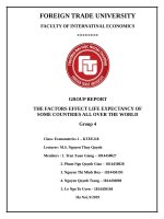
 Signal 1: Using qualitative methods (visual methods)

Graph of ei according to BUSTRAVL

Comment: From the graph, the values on the graph are not evenly distributed

Have the sign of disease error variance
 Signal 2: UsingWhite-test
- Conduct regression of sub-model:
e2i = α1 + α2. FARE + α3. INCOME + α4. POP + α5. FARE 2 + α6. FARE. INCOME + α7. FARE. POP + α8INCOME2 + α9. INCOME. POP +
α10. POP2 + vi

12


- The result shown in the table:
White's test for heteroskedasticity
OLS, using observations 1-40
Dependent variable: uhat^2
coefficient
std. error
--------------------------------------------------------------const
5,19333e+06
8,74264e+06
FARE
−1,84745e+06

6,22686e+06
INCOME
−455,497
949,072
POP
2455,89
5105,07
sq_FARE
−1,84226e+06
2,16245e+06
X2_X3
297,210
368,212
X2_X4
116,104
734,557
sq_INCOME 0,00541227
0,0259041
X3_X4
−0,112996
0,319942
sq_POP
−0,0440935
0,207512

t-ratio

p-value

0,5940

−0,2967
−0,4799
0,4811
−0,8519
0,8072
0,1581
0,2089
−0,3532
−0,2125

0,5570
0,7687
0,6348
0,6340
0,4010
0,4259
0,8755
0,8359
0,7264
0,8332

Unadjusted R-squared = 0,145698
Test statistic: TR^2 = 5,827904,
with p-value = P(Chi-square(9) > 5,827904) = 0,757011
Exhibit 12. Testing error variance with the quantitive method White-test
(Source: we calculated it based on the statistic in the Gretl software)
- Hypothesis: {

H0: PSSS unchanged

H1: PSSS changed

- p-valute = 0.757011 > 5% so reject H0



The model suffers from PSSS at 5% significant level

* Solution: Using verification Robust
Model 5: OLS, using observations 1-40 Independent variable: BUSTRAVL
Heteroskedasticity-robust standard errors, variant HC1
const
FARE
INCOME
POP

Coefficient
2683,59
−609,126
−0,116272
1,88836

Std. Error
1325,57
506,205
0,0668052
0,0890323

t-ratio
2,024

−1,203
−1,740
21,21

p-value
0,0504
0,2367
0,0903
<0,0001

*
*
***

13


Mean dependent var
Sum squared resid
R-squared
F(3, 36)
Log-likelihood
Schwarz criterion

1933,175
27674784
0,880001
172,0801
−325,7006
666,1567

S.D. dependent var
S.E. of regression
Adjusted R-squared
P-value(F)
Akaike criterion
Hannan-Quinn

2431,757
876,7805
0,870001
2,14e-21
659,4012
661,8438

Recalibrating the model (used Robust Test) by White test, we get the following results:
White's test for heteroskedasticity
OLS, using observations 1-40
Dependent variable: uhat^2
coefficient
std. error
--------------------------------------------------------------const
5,19333e+06
8,74264e+0
6
FARE
−1,84745e+06
6,22686e+0
6
INCOME

−455,497
949,072
POP
2455,89
5105,07
sq_FARE
−1,84226e+06
2,16245e+0
6
X2_X3
297,210
368,212
X2_X4
116,104
734,557
sq_INCOME
0,00541227
0,0259041
X3_X4
−0,112996
0,319942
sq_POP
−0,0440935
0,207512

t-ratio

p-value

0,5940

0,5570

−0,2967

0,7687

−0,4799
0,4811
−0,8519

0,6348
0,6340
0,4010

0,8072
0,1581
0,2089
−0,3532
−0,2125

0,4259
0,8755
0,8359
0,7264
0,8332

Unadjusted R-squared = 0,145698
Test statistic: TR^2 = 5,827904,
with p-value = P(Chi-square(9) > 5,827904) = 0,757011

- Hypothesis: {

H0: PSSS unchanged

H1: PSSS changed

- p-valute = 0.757011 > 5%, so rejectH0

The model still suffers from PSSS at 5% significant level
However, because the Robust test has controlled the error variance, we can still use the
model after the Robust without affecting the deductive.

14


4.2.2. Discussion
The model we used to interpret is:
BUSTRAVEL = 2683.59 – 609.126.FARE – 0.116272.INCOME + 1.88836.POP (1)
From the above model estimation, tests and solutions, we have drawn the best model
available:
BUSTRAVEL = 2683.59 – 609.126.FARE – 0.116272.INCOME + 1.88836.POP (2)
Model (2) has been applied with Robust to control the error: Heteroscedasticity


Model (1) has the error: Heteroscedasticity.



For the Heteroscedasticity, our team implemented Robust test and obtained the
model (2), although it could not fix the errors but was controlled and the model

could still be used to infer without being affected by errors.



The used model is consistent with economic theory. Firstly, taking bus is a
secondary commodity, so when the income of passenger increases to a certain
extent and bus fare increases they tend to reduce bus consumption , instead, they
use other alternative means such as motorcycles, taxis, cars,... Therefore, the
regression coefficients of the two variables INCOME, negative FARE are
appropriate. Secondly, with the growth of population, more and more people using
bus as a means of transportation is reasonable, so the regression coefficient of
positive POP variables is appropriate.



The significance level of the model is 88,0001%, although not higher than 95% but
this level of significance is quite high and this is the best current model.

15


CONCLUSION
In conclusion, basing on the theoretical basis mentioned in part 2 and on the
basis of using Gretl in running models and making tests, we analyzed and made
relatively complete remarks on the influence of each factor: bus fares, income and
population on the level of using bus as a means of transportation in the urban areas.
We think, through the above analysis, we can help policymakers to put in the right
amount of buses to service. In fact, there are many other factors that affect the level
of bus traffic in urban areas, but due to limited time and capacity, our research only
focuses on three variables: bus fares, income and population. Therefore, we can’t

fully reflect all faces of the problem. If possible, we should study some more
explanatory variables such as gasoline prices, prices of alternative vehicles such as
motorcycles, cars or the level of satisfaction of people when they take the bus.
Again, due to the limitation of understanding and resources, our report may
contain misinterpretations. We hope that Dr. Tu Thuy Anh and readers can give us
constructive comments on the report so that we would improve ourselves and do
better in the future.
Sincerely.

16


REFERENCES
1. Textbook Introduction to Econometrics, Brief edition, James H.Stock and Mark
W.Waston
2. Gretl software, Ramanathan Data 4-4
3. Website:
 /> />