An efficient algorithm for mining high utility association rules from lattice
Bạn đang xem bản rút gọn của tài liệu. Xem và tải ngay bản đầy đủ của tài liệu tại đây (1.41 MB, 14 trang )
Journal of Computer Science and Cybernetics, V.36, N.2 (2020), 105–118
DOI 10.15625/1813-9663/36/2/14353
AN EFFICIENT ALGORITHM FOR MINING HIGH UTILITY
ASSOCIATION RULES FROM LATTICE
TRINH D.D. NGUYEN1,∗ , LOAN T.T. NGUYEN2,3 , QUYEN TRAN4 , BAY VO5
1 Faculty
2 School
of Computer Science, University of Information Technology,
Ho Chi Minh City, Vietnam
of Computer Science and Engineering, International University,
Ho Chi Minh City, Vietnam
3 Vietnam
4 Informatics
5 Faculty
National University, Ho Chi Minh City, Vietnam
Team, Bac Lieu Specialized High School Bac Lieu City, Vietnam
of Information Technology, Ho Chi Minh City University of Technology,
Ho Chi Minh City, Vietnam
Abstract. In business, most of companies focus on growing their profits. Besides considering profit
from each product, they also focus on the relationship among products in order to support effective
decision making, gain more profits and attract their customers, e.g. shelf arrangement, product displays, or product marketing, etc. Some high utility association rules have been proposed, however,
they consume much memory and require long time processing. This paper proposes LHAR (Latticebased for mining High utility Association Rules) algorithm to mine high utility association rules based
on a lattice of high utility itemsets. The LHAR algorithm aims to generate high utility association
rules during the process of building lattice of high utility itemsets, and thus it needs less memory and
runtime.
Keywords. High utility itemsets; High utility itemset lattice; High utility association rules.
1.
INTRODUCTION
The frequent itemset mining (FIM) only supports to find frequent itemsets in transaction
database. The problem only considers the appearance of items in each transaction instead of
their profit, means that each item has similar utility (profit). In the real world of transaction
database, the profits of items are different [18]. For example, in a transaction, customer may
buy 10 bottles of water and one bottle of wine, however, the profit from a bottle of wine may
be much higher than that of water even the quantity of bottles of water is higher. To solve the
problem, high utility itemset mining (HUIM) has been investigated in order to consider the
frequent of each item in itemsets as well as their utility value. The result of HUIM has been
applied applied to many different fields, e.g. clicks on website, website marketing, retails,
medical, etc. [18]. In HUIM, high utility association rules play an important part to consider
the relationship among items in database. However, there have not been many researches
on high utility association rules. Two algorithms, HGB-HAR (High-utility Generic Basis High-utility Association Rule) [12] and LARM (Lattice-based Association Rules Miner) [10]
*Corresponding author.
E-mail addresses: (T.D.D.Nguyen);
(L.T.T.Nguyen); (Q.Tran);
(B.Vo).
c 2020 Vietnam Academy of Science & Technology
106
TRINH D.D. NGUYEN, et al.
have been proposed. The LARM algorithm has better performance than that of HGB-HAR.
However, LARM is based on a two-stages process to generate high utility association rules
(HARs), the first stage is to build high utility itemsets lattice, and the second is to generate
HARs from the built lattice. Thus, LARM still has longer execution time and consumes
more memory. This paper aims to improve the performance of LARM for mining HARs
from high utility itemsets lattice (HUIL). The main contributions are as follows:
− Propose LHAR (Mining High utility Association Rules based on building Lattice)
algorithm to mine high utility association rules during the processing of building high
utility itemsets lattice.
− Carry out experiments on different databases to indicate the efficiency of LHAR algorithm comparing to LARM algorithm. The rest of the paper is organized as follows:
Section 2 presents definitions and states the problem of mining high utility association
rules. Section 3 collects recent related researches on mining HUIs and HARs. Section 4
discusses new algorithm, LHAR, to mine HARs based on HUIL. Section 5 presents the
comparison between LHAR algorithm and LARM [10] algorithm in terms of runtime
and memory usage. Section 6 concludes and discusses future works.
2.
DEFINITIONS
Definition 2.1. (Transaction database) [10]. Given a finite set of items I. A transaction
database D is a set of finite transactions, D = {T1 , T2 , ..., Tn }, in which each transaction Td
is a subset of I and has a unique identifier (Transaction identifier - Tid). Each item ip in Td
is associated to a positive number, called quantity, denoted as q(ip , Td ). Each item ip ∈ I in
Td has a utility value, denoted as p(ip ).
Table 1. Transaction Database example
TID
T1
T2
T3
T4
T5
Transaction
A(4)C(1)E(6)F (2)
D(1)E(4)F (5)
B(4)D(1)E(5)F (1)
D(1)E(2)F (6)
A(3)C(1)E(1)
Unit profit
A(4)C(5)E(1)F (1)
D(2)E(1)F (1)
B(4)D(2)E(1)F (1)
D(2)E(1)F (1)
A(4)C(5)E(1)
Table 1 describes an example of transaction database with five transactions T1 , T2 , ..., T5 .
Considering transaction T2 , it has three items D, E, F with corresponding quantity 1, 4, 5
and their corresponding utility 2, 1, 1.
Definition 2.2. (Utility of an item in a transaction) The utility of an item i in a transaction
Td is denoted as u(i, Td ) and is defined as p(i) × q(i, Td ). For example, the utility of item D
in transaction T2 in the above sample database is u(D, T2 ) = 2 × 1 = 2.
Definition 2.3. (The utility of an itemset in a transaction) The utility of an itemset X in
a transaction Tc , denoted as u(X, Tc ), and is defined as u(X, Tc ) =
u(i, Tc ), X ⊆ Tc . For
i∈X
107
AN EFFICIENT ALGORITHM FOR MINING
example, the utility of itemset X = {D, E} in T2 from the above sample database in Table
1 is u({D, E}, T2 ) = u(D, T2 ) + u(E, T2 ) = 2 + 4 = 6.
Definition 2.4. (The utility of an itemset in database) The utility of an itemset X in
database D is calculated as the sum utility of X in all transactions containing X, that is
u(X) =
u(X, Td ). The utility of itemset X = {E, F } in database D is u(X) = 31.
X⊆Td ∧Td ∈D
Definition 2.5. (The support of an itemset in database) The support of itemset X in
database D indicates the frequency of availability of X in D. The support value of X with
respect to D is defined as the proportion of itemsets in a database containing X. The support
of X = {A, C, E} in the above database is supp({A, C, E}) = 2/5 or supp({A, C, E}) = 2,
in short.
Definition 2.6. (High utility itemset) An itemset X is considered as a high utility itemset
if its utility u(X) is no less than a minimun utility threshold (minU til) defined by user
(u(X) ≥ minU til). Otherwise, X is called a low utility itemset.
Definition 2.7. (Local utility value of an item in an itemset). The local utility value
of an item xi in itemset X, denoted as luv(xi , X), and is defined by the sum of utility
of xi in all transactions containing X. The formula to calculate luv(xi , X) is luv(xi , X) =
u(xi , Td ). For example, the local utility of xi = {E} in X = {E, F } is luv(xi , X) =
X⊆Td ∧Td ∈D
6 + 4 + 5 + 2 = 17.
Definition 2.8. (Local utility value of itemset in itemset) The local utility value of itemset
X in itemset Y, X ⊆ Y , denoted as luv(X, Y ), and is defined by the sum of local utility of
luv(xi , Y ).
each item xi ∈ X in Y . The formula is described as follows luv(X, Y ) =
xi ∈X⊆Y
For example, luv(X, Y ) of X in Y where X = {D, E} and Y = {D, E, F } (given in Table 1)
is luv(X, Y ) = (2 + 2 + 2) + (4 + 5 + 2) = 6 + 11 = 17.
Definition 2.9. (High utility association rule). A high utility association rule R having the
form of X → Y \ X, describes the relationship of two high utility itemsets X, Y ⊆ I, X ⊂
Y . The utility confidence of R, uconf (R), is denoted as uconf (R) = luv(X, XY )/u(X).
The association rule R : X → Y is called the high utility association rule if uconf (R) is
greater than or equal to a minimum utility confidence threshold (minU conf ) given by user.
Otherwise, R is considered as low utility association rule. For instance, X = {F [14], E[17]}
and itemset Y = {D[6], F [12], E[11]}, the rule R : F E → D (which is the shortened form
of R : F E → DF E \ F E) has confident value uconf (R) = 23/31 × 100 = 74.19%. If
minU conf = 60%, then R is considered as high utility association rule.
3.
3.1.
RELATED WORK
High utility itemset mining
The HUIM problem was first introduced in 2004 by Yao et al. [15] and has since, attracted various researchers recently. HUIM addresses the realistic problem that each item
can be occurred more than once in each transaction and has its own utility values. Liu
et al. (2005) proposed the Two-Phase algorithm [9], one of the earliest algorithms for mining high utility itemsets. The Two-Phase algorithm presented and applied the definition
108
TRINH D.D. NGUYEN, et al.
of Transaction Utility (TU) and Transaction Weighted Utility (TWU) onto the Apriori algorithm [1] to mine HUIM efficiently and accurately. However, Two-Phase generates a large
number of candidates in its first phase by over-estimating the utility of candidates. Besides,
it performs multiple database scans and thus consumes a large amount of memory and need
long execution time.
The Two-Phase algorithm as said, can find the complete set of HUIs in transaction
database, but it still is a computationally expensive algorithm. Thus, several approaches
haven been proposed to increase further the performance of HUIM. Le et al. introduced two
new algorithms named TWU-Mining [6] and DTWU-Mining [7]. The proposed algorithms
aim to reduce the candidates generated when mining for HUI using TWU measure by using
the data structures, the IT-Tree [17] and the WIT-Tree [7]. Another algorithm named UPGrowth, which was proposed by Tseng et al. [14], introduced a novel tree structure called
UP-Tree, to efficiently mining HUIs. The UP-Growth algorithm consisting of two stages,
is based on the FP-Growth algorithm [4] and the down-ward closure property of the TwoPhase algorithm [9]. Tseng et al. proposed four effective strategies for pruning candidates:
i) Discarding global unpromising items (DGU); ii) Decreasing global node utilities (DGN);
iii) Discarding local unpromising items (DLU); iv) Decreasing local node utilities (DLN). By
applying these strategies during the process of building global and local UP-Tree, UP-Growth
generates less candidates than the Two-Phase algorithm does. And thus, the runtime of UPGrowth has 1000 times faster than that of Two-Phase. Besides, it also requires less memory
than Two-Phase. However, UP-Growth still generates a large number of candidates in its
first phase by over-estimating utility of each candidates. Moreover, building and maintaining
the UP-Tree structure is computationally expensive. The improved version of UP-Growth,
named UP-Growth+, was also proposed by Tseng et al. in 2013 [13]. UP-Growth+ came
with two new strategies to optimize further the UP-Tree, called Discarding local unpromising
items and their estimated Node Utilities and Decreasing local Node utilities for the Nodes.
In 2014, Yun et al. proposed the MU-Growth [16] algorithm to improve the UP-Growth+
algorithm. MU-Growth came with another tree data structure called MIQ-Tree (Maximum
Quantity Item Tree). In 2014, Fournier-Viger et al. has introduced a more efficient pruning
strategy, named Estimated Utility Co-occurrence Pruning (EUCP) [3], to help speeding
up the process of mining HUIs. EUCP makes use of the Estimated Utility Co-occurrence
Structure (EUCS) to consider item co-occurrences.
Zida et al. proposed EFIM algorithm [18] for mining HUIs effectively with two new
upper bounds on utility: Revised sub-tree utility (SU) and local utility (LU). The author
demonstrated that the two proposed upper bounds are tighter than TWU and remaining
utility based upper bound. EFIM algorithm also introduced two new strategies, High-utility
Database Projection (HDP) and High-utility Transaction Merging (HTM), to reduce the cost
of scanning database. Unlike Two-Phase or UP-Growth, EFIM is a single phase algorithm.
And by utilising the newly proposed upper bounds and strategies, EFIM has better execution
time and consume less memory than previous approaches.
In 2017, Krishnamoorthy make use of all existing pruning techniques, such as TWUPrune [9], EUCS-Prune [3], U-Prune [8] to develop two more pruning techniques, named
LA-prune and C-prune. These pruning strategies were then incorporated into an algorithm
called HMiner [5].
As in 2019, an extended version of EFIM was proposed by Nguyen et al. [11], named
AN EFFICIENT ALGORITHM FOR MINING
109
iMEFIM, which utilized the P-set data structure to reduce the cost of database scans and
thus boost the overall performance of the EFIM algorithm dramatically, and iMEFIM also
adapted a new database format to handle dynamic utility values to be able to mine HUIs in
real-world databases [11].
3.2.
Mining high utility association rules from high utility itemsets
Sahoo et al. proposed the HGB-HAR algorithm [12] for mining HARs from high utility
generic basic (HGB). The algorithm consists of three phases: (1) mining high utility closed
itemsets (HUCI) and generators; (2) generating high utility generic basic (HGB) association
rules; And (3) mining all high utility association rules based on HGB. The HGB-HAR
algorithm [12] is one of the first high utility association rule mining algorithm. However, the
phase 3 of this approach requires more execution time if the HGB list is large and each rule
in HGB contains many items in both antecedent and consequent. In this paper, to address
this issue, we propose an algorithm for mining high utility association rules using a lattice.
Mai et al. proposed LARM algorithm [10] for mining HARs from high utility itemsets
lattice (HUIL). The algorithm has 2 phases: (1) building a HUIL from the discovered set of
high utility itemsets; And (2) mining all high utility association rules (HARs) from HUIL.
The LARM algorithm is more efficient compared to HGB-HAR in terms of memory usage
and runtime. However, this algorithm has two depth scan processes through ResetLattice
and InsertLattice. Besides, the algorithm is only able to generate HARs after having the
complete lattice of high utility itemsets.
4.
PROPOSED METHOD
Problem statement: Given a transaction database D, minimum utility threshold minU til
and minimum confidence threshold minU conf . The problem of mining all high utility
association rules from database D is to generate all association rules, formed from two
high utility itemsets having utility value greater than or equal to minU til, and having
uconf (R) ≥ minU conf .
4.1.
LHAR (Lattice-based for mining High utility Association Rules) algorithm
In this paper, we propose an efficient approach to mine all high utility association rules
based on high utility itemsets lattice. The overall process is consisted of two phases, as
follows:
− Phase 1. Mine the complete set of HUIs having utility value greater than or equal to
minUtil from database D. In this stage, the EFIM algorithm [18] is used, which is the
most efficient HUIM algorithm.
− Phase 2. Construct HUIL and mine HARs during the HUIL construction process.
This process only requires a single step, compared to the two steps from the LARM
algorithm, and thus significantly reduces the overall execution time and memory consumption.
The main contribution of this paper is in Phase 2. In this stage, instead of performing two
separated steps, which are constructing the lattice first and then scan the constructed lattice
110
TRINH D.D. NGUYEN, et al.
the discover HARs as in the LARM algorithm does, we group these steps into a single stage.
In which, while constructing the HUIL, we directly extract the high-utility association rules
from the lattice if the rules satisfy the minUconf threshold. This help significantly reduce
the runtime required to mine the complete set of HARs. Evaluation studies have shown
that our approach has the execution time outperforming the original LARM algorithm over
a thousand-fold and dramatically reduces memory usage, up to half of LARM.
Pseudo-code of our approach is presented in Section 4.2 and is named LHAR. The
LHAR algorithm is level-wise and contains two main functions, the BuildLattice and the
InsertLattice functions, where, the BuildLattice function is called to construct the HUIL
based on the input set of HUIs and a user-specified minU conf threshold. Note that the HUIs
were ascending sorted by the number of items in each HUI (called level). The BuildLattice
first initializes the Root node of the lattice and the set of discovered rules (RuleSet). Then
at each level of the lattice, the InsertLattice is then called to insert an itemset X into the
lattice and to recursively explore subsets of X which are HUIs to directly discover and extract
HARs during the construction process, non-HARs are also pruned directly during the HUIL
construction. By using this approach, we completely eliminated the need of rescanning the
constructed lattice to extract HARs, which is time and memory consuming. Memory usage
is now only for storing the discovered rules and the partially constructed HUIL. Section 4.2
presents the LHAR algorithm in details.
Figure 1. High utility itemsets lattice
The constructed HUI lattice of the sample database in Table 1 is presented in Figure 1.
This lattice is similar to that from LARM [12] including a root node and parent-child nodes. The root node is a node containing the empty itemset and has no utility value (or
utility equals to 0). Each node (non-root nodes) contains a HUI along with its utility
and support value. For instance, considering node A[28](28, 2), the itemset is A, its associated values are U tility = 28, Support = 2. Node A[28](28, 2) is the parent of node
A[28]C[10](38, 2) which contains two items A and C with the corresponding utility values are
AN EFFICIENT ALGORITHM FOR MINING
111
U tility(A) = 28, U tility(C) = 10. The utility value and support of AC are U tility =
38, Support = 2, respectively. In another words, node A[28]C[10](38, 2) is the child of
A[28](28, 2). And A[28](28, 2) has two children, A[28]C[10](38, 2) and A[28]E[7](35, 2).
Figure 1 shows the HUIL constructed from the list of HUIs mined from the sample
database with minU til threshold equals to 23 (25% of the total utility of the transaction
database example).
4.2.
LHAR algorithm
This section presents the pseudo code of the proposed LHAR algorithm. The inputs of
the algorithm are the complete set of discovered HUIs (T ableHU I), ascending sorted by the
number of items, and the user-specified minU conf threshold.
The algorithm returns the complete set of mined HARs from the input and satisfied the
minU conf threshold.
LHAR algorithm
Input : TableHUI , minUconf
Output : RuleSet ;
01: BuildLattice ( tableHUI , minUconf )
02: SET rootNode =∅;
03: SET RuleSet =∅;
04: SET Root = new Itemset (0 ,0);
05: rootNode . add ( Root );
06: FOR EACH ( level in tableHUI . getLevels )
07:
FOR EACH ( X in level )
08:
Root . isTraversed = false ;
09:
SET resetList = ArrayList of Empty Itemset ;
10:
InsertLattice (X , Root , minUconf );
11:
FOR EACH ( Y in resetList )
12:
Y . isTraversed = false ;
13:
END FOR
14:
END FOR
15: END FOR
16: END
17: InsertLattice (X , rNode , minUconf )
18:
IF rNode . isTraversed THEN
19:
return ;
20:
END IF
21: SET Flag = true , rNode . isTraversed = true ;
22: IF X . size >1 THEN
23:
FOR EACH ChildNode IN rNode . ChildNode
24:
IF ChildNode ⊂ X THEN
25:
IF ChildNode . isTraversed = false THEN
26:
resetList . add ( ChildNode );
27:
Uconf = R . C a lc u l at e C on f i de n c e ( ChildNode , X );
28:
IF Uconf ≥ minUconf THEN
29:
SET R : ChildNode → X\ChildNode ;
30:
RuleSet . add ( R );
31:
END IF
32:
END IF
33:
Set Flag = false ;
112
TRINH D.D. NGUYEN, et al.
34:
InsertLattice (X , ChildNode , minUconf );
35:
END IF
36:
END FOR
37: END IF
38: IF Flag THEN
39:
IF X . isTraversed = false THEN
40:
rootNode . add ( X );
41:
rNode . ChildNode . add ( X );
42:
resetList . add ( X );
43:
X . isTraversed = true ;
44:
END IF
45:
ELSE
46:
rNode . ChildNode . add ( X );
47:
END ELSE
48: END IF
This section explains how the LHAR algorithm mines HARs from HUIs.
∗ Initially, the algorithm triggers BuildLattice method to construct a lattice with rootN ode :
Root(0, 0) and initiates the result collector RuleSet (line 2, 3).
∗ Next, the algorithm scans HUIs, which were ascending sorted by the number of items
(level). Considering a HUI {X}, the flag isT raversed is used to track if {X} is traversed (true) or not (f alse). isT raversed is initiated for root node Root(0, 0) as f alse. An
empty resetList is used at line 9 to handle HUIs which has isT raversed = true during
the lattice construction. The algorithm then calls InsertLattice(X, Root, minU conf )
to insert {X} into rootN ode and generate HARs which satisfy minU conf (line 10).
Line 11 and 12 is called to reset the flag isT raversed for each HUI in resetList to false
after finish processing InsertLattice(X, Root, minU conf ) on each node {X}.
The execution of InsertLattice(X, rN ode, minU conf ) is as follows.
∗ It first checks the value of isT raversed on the rN ode parameter. If the value is f alse,
then the method will perform the following steps set F lag value to true. The F lag
variable is used to check if {X} can be inserted into rN ode. Set isT raversed of
rN ode to true to notify that rN ode is already processed. InsertLattice is then called
recursively to decide which node will be the parent of {X}.
∗ Next, the method checks the size of itemset {X}, if {X} has only one item, then it
adds {X} directly into rootN ode (line 38). The steps to add {X} into rN ode are
described from line 38 to 48. If {X} does not exist in the rootN ode then adds it into
lattice as the child of rootN ode. Otherwise, {X} is added into rN ode. If the size of
{X} is greater than one, it scans each child node ChildN ode of rN ode. If ChildN ode
is the child of {X} (ChildN ode ⊂ {X}) then (i) it checks if isT raversed of ChildN ode
is f alse in order to add ChildN ode into resetList (line 24, 25); (ii) it then considers
the rule R : ChildN ode → X \ ChildN ode (line 27) and calculate the confidence value
U conf of R, and then add R into RuleSet if U conf ≥ minU conf (line 28); (iii) it
recursively calls InsertLattice method to process the insertion of {X} into ChildN ode
(line 34).
AN EFFICIENT ALGORITHM FOR MINING
4.3.
113
LHAR algorithm illustrations
Consider the sample database given in Table 1, using minU til = 23 and minU conf =
60%. The list of HUIs generated by the EFIM algorithm [18], sorted by levels, are as follows:
- Level-1:
{A[28](28, 2)}, denoted as {A}.
- Level-2:
{A[28]C[10](38, 2),
A[28]E[7](35, 2),
F [14]E[17](31, 4)}, denoted as {AC, AE, F E}.
- Level-3:
{B[16]D[2]E[5](23, 1),
D[6]F [12]E[11](29, 3),
A[16]C[5]F [2](23, 1),
A[28]C[10]E[7](45, 2),
A[16]F [2]E[6](24, 1)} denoted as {BDE, DF E, ACF, ACE, AF E}.
- Level-4:
{B[16]D[2]F [1]E[5](24, 1),
A[16]C[5]F [2]E[6](29, 1)}, denoted as {BDF E, ACF E}.
The LHAR algorithm processes the list of HUIs generated by EFIM to construct HUI
lattice and mine for HARs:
∗ Initially, this algorithm declares a lattice with rootN ode, and defines an empty RuleSet.
∗ It then processes level1 HUIs. Consider {X} = {A} ∈ level1. {X} is added into
rootN ode. The RuleSet is still empty since no rules were generated.
∗ Next, considering level2 HUIs. For each {X} ∈ level2, {AC} and {AE} is then added
into {A} as children. {F E} is added directly into Root(0, 0) since it has no parent which
are 1-itemsets. Considering the itemset {AC}, in which ChildN ode = {A}, X = {AC},
and ChildN ode ⊂ X, we have found a rule R : A → AC \ A ⇔ R : A → C, R has
U conf (R) = 100% ≥ minU conf , R is then added into RuleSet. Similarly, with
X = {AE} and ChildN ode = {A}, R : A → AE \ A ⇔ R : A → E is then added into
RuleSet.
∗ At level3, considering X = {BDE}, {DF E}, {ACE}, {ACF } and {AF E}, no rules
were generated for X = {BDE}.
− With X = {DF E} we have ChildN ode = {F E}, thus R : F E → DF E \
F E ⇔ R : F E → D is added into the RuleSet since its U conf (R) = 74.19% ≥
minU conf .
− With X = {ACE}, ChildN ode = {A}, we have R : A → ACE \ A ⇔ R : A →
CE, U conf (R) = 100% ≥ minU conf , R is added into RuleSet. InsertLattice
then recursively processes ChildN ode = {AC} and {AE}, we have R : AC →
ACE \ AC ⇔ R : AC → E, U conf (R) = 100% ≥ minU conf , R is added into
RuleSet. We also have R : AE → ACE \ AE ⇔ R : AE → C, U conf (R) =
100% ≥ minU conf , R is added into RuleSet.
114
TRINH D.D. NGUYEN, et al.
Table 2. Discovered HARs from D using minU til = 23, minU conf = 60%
Rules
1. A → C
2. A → E
3. F E → D
4. A → CE
U conf (%)
100
100
74.19
100
Rules
5. AC → E
6. AE → C
7. AE → F
8. BDE → F
U conf (%)
100
100
62.86
100
Rules
9. ACF → E
10. ACE → F
11. AE → CF
12. AF E → C
U conf (%)
100
60
62.86
100
− With X = {ACF }, ChildN ode = {A}, we have R : A → ACF \ A ⇔ R : A →
CF , U conf (R) = 57.14% < minU conf , thus we discard this rule. At this itemset, InsertLattice is then called recursively to process ChildN ode = {AC}, we
have R : AC → ACF \ AC ⇔ R : AC → F , U conf (R) = 55.26% < minU conf ,
thus we discard this rule.
− The remaining itemset is X = {AF E}, ChildN ode = {A}, we have R : A →
AF E \ A ⇔ R : A → F E, U conf (R) = 57.14% < minU conf , R is discarded.
InsertLattice then processes recursively to ChildN ode = {AE} and {F E}.
With ChildN ode = {AE}, we have R : AE → AF E \ AE ⇔ R : AE → F ,
U conf (R) = 62.86% ≥ minU conf , R is added into RuleSet. With ChildN ode =
{F E}, we have R : F E → AF E \ F E ⇔ R : F E → C, U conf (R) = 25.81% <
minU conf , R is then discarded.
∗ The process continues similarly with level-4 HUIs, which are {BDF E} and {ACF E}.
The HARs found at this level are BDE → F, ACF → E, ACE → F, AE → CF and
AF E → C. The discarded rules are DF E → B, AC → F E and F E → AC with the
U conf (R) = {27.59%, 55.25%, 25.81%}, respectively.
The results of the algorithm are presented in Table 2 in the order of discovery, including
the discovered rules and the associated U conf (R) values.
4.4.
The advantages of LHAR algorithm
LHAR algorithm has the following improvements compared to the LARM algorithm [10],
which helps increase the performance of the algorithm in terms of runtime and memory usage.
∗ LHAR constructs a lattice of high utility itemsets with rootN ode then apply a single
depth scan by InsertLattice, while LARM does the process through two separated
methods ResetLattice and InsertLattice. The method ResetLattice requires a similar
amount of execution time to InsertLattice.
∗ LHAR combines the process of building lattice and generating HARs into one process.
It bypasses the method F indHuiRulesF romLattice from the LARM algorithm. As a
result, LHAR has better runtime and consumes less memory.
115
AN EFFICIENT ALGORITHM FOR MINING
Table 3. Test datasets and their characteristics
Dataset
Chess
Mushroom
Accidents
N ◦ trans
3,196
8,124
340,183
N ◦ items
75
119
468
Total utility
2,156,659
3,413,720
196,141,636
Size (KB)
642
1,064
64,686
Table 4. The number of HUIs and HARs discovered from test datasets
Dataset
Chess
Mushroom
Accidents
minU til%
24.5
25.5
26.5
27.5
10
11
12
13
10
11
12
13
5.
5.1.
◦
N HUIs
9,740
4,226
1,911
791
707,250
5,800
2,726
1,152
7,479
2,367
728
189
N ◦ HARs minU Conf
40%
60%
80%
1,803,478 1,691,473 593,668
490,292
476,465 200,900
132,873
132,250
703,86
30,726
30,726
22,211
700,455
679,987 594,178
281,150
279,574 255,553
78,308
78,308
74,688
19,606
19,606
19,474
729,209
422,415 100,614
131,644
88,388
23,911
22,510
17,778
5,568
2,623
2,453
1,024
EXPERIMENTAL STUDIES
Datasets and experimental environment
We used the datasets from an open-source website SPMF by Fournier [2]:
These datasets have been used in many publications in the fields
of data mining, high utility itemset mining and high utility association rule mining. The attributes of these datasets are described in UCI Machine Learning Repository at:
Table 3 shows characteristics of the datasets used in our tests.
The LARM and LHAR algorithm were all developed using Java. The algorithms were
experimented on a computer with the configuration as follows: Intel R CoreTM i7-8550U
processor, clocked at 1.80GHz, 8 GB of RAM, and running Windows 10 Professional 64-bit.
The number of HUIs and HARs mined from relevant datasets are presented in Table 4.
5.2.
Comparison on runtime and memory usage between LARM algorithm and
LHAR algorithm
We thoroughly analyze the performance between of LHAR algorithm and LARM algorithm on different datasets, and the minUconf threshold was fixed at 60% on all the datasets.
In general, the running time and memory consumption of the LHAR algorithm are significantly better than those of the LARM algorithm [10] (Figures 2 to 4).
In the Chess dataset evaluations, it can be seen that the execution time of LHAR has
116
TRINH D.D. NGUYEN, et al.
a major speed boost (Figure 2), which is up to 1400 times faster than LARM, it took only
almost 4 seconds for LHAR to finish the task at minU til = 24.5% while LARM needs an hour
and a half on the test computer to complete. This is the biggest difference in runtime between
LHAR and LARM in our studies. For memory usage on the Chess dataset (Figure 2), LHAR
reduces the memory needed by half on all minUtil thresholds, LHAR requires the maximum
amount 550MB of memory at minU til = 24.5% while LARM needed over 1GB of memory.
The execution time of LHAR on the Mushroom dataset (Figure 3) is also lower than that
of LARM with the speed up factor is approximately 33 times at minU til = 10%. As the
minimum utility threshold decrease from 13% down to 10%, the increasing in the runtime of
LHAR is almost linear while LARM has a sharp increase here. And for the memory usage
comparison, the same thing as on the Chess dataset, the memory utilization of LHAR on
Mushroom is better than LARM (Figure 3) on all thresholds tested.
Figure 2. Runtime and memory comparison on Chess dataset
We repeated our process, this time on the Accidents dataset. In this test, the speed up
factor is approximately 520 times at minU til = 10% (Figure 4) and is also almost linear.
For memory consumption, which is also shown in Figure 4, LHAR is still a winner here with
twice the times lower memory usage than LARM, with the maximum value at 320MB when
compared to almost 640MB of LARM at the same minU til.
Through out the evaluation studies, it can be seen that the LHAR algorithm has superior
performance in both runtime and memory utilization when compared to that of LARM, with
the speed up factor is up to 1400 times and memory usage is two times lower than LARM.
Figure 3. Runtime and memory comparison on Mushroom dataset
AN EFFICIENT ALGORITHM FOR MINING
117
Figure 4. Runtime and memory comparison on Accidents dataset
The lower minUtil threshold, the higher speed up factor. This also shows that the increasing
in execution time of LHAR is almost linear when we dropped the minU til threshold on all
the tests.
6.
CONCLUSIONS
Based on the research of mining HARs from HUIL in LARM algorithm [10], we proposed
an improvement of LARM via our algorithm LHAR, in which mines HARs during HUIL
construction progress, aims to reduce the algorithm execution time and memory consumption. We conducted variety of experiments on standard databases to firm that LHAR is more
efficient than LARM in terms of runtime and memory usage. LHAR algorithm is useful for
decision systems and management boards in many fields, e.g., business, education, medical,
stocks, etc. This approach can be extended further to mine low high utility association rules,
which has tentative support for organization to improve their business activities.
ACKNOWLEDGMENT
This research is funded by Vietnam National Foundation for Science and Technology
Development (NAFOSTED) under grant number 102.05-2018.01.
REFERENCES
[1] R. Agrawal and R. Srikant, “Fast algorithms for mining association rules in large databases,” in
Proceedings of the 20th International Conference on Very Large Data Bases, 1994, pp. 487–499.
[2] P. Fournier-Viger, A. Gomariz, T. Gueniche, A. Soltani, C.-W. Wu, and V. S. Tseng, “SPMF:
A java open-source pattern mining library,” The Journal of Machine Learning Research, vol. 15,
no. 1, pp. 3389–3393, jan 2014.
[3] P. Fournier-Viger, C. W. Wu, S. Zida, and V. S. Tseng, “FHM: Faster high-utility itemset mining
using estimated utility co-occurrence pruning,” International Symposium on Methodologies for
Intelligent Systems, vol. 8502 LNAI, pp. 83–92, 2014.
[4] J. Han, J. Pei, Y. Yin, and R. Mao, “Mining frequent patterns without candidate generation:
A frequent-pattern tree approach,” Data Mining and Knowledge Discovery, vol. 8, no. 1, pp.
53–87, 2004.
118
TRINH D.D. NGUYEN, et al.
[5] S. Krishnamoorthy, “HMiner: Efficiently mining high utility itemsets,” Expert Systems with
Applications, vol. 90, pp. 168–183, 2017.
[6] B. Le, H. Nguyen, T. Cao, and B. Vo, “A novel algorithm for mining high utility itemsets,”
in Proceedings of 2009 1st Asian Conference on Intelligent Information and Database Systems,
ACIIDS 2009, 2009, pp. 13–17.
[7] B. Le, H. Nguyen, and B. Vo, “An efficient strategy for mining high utility itemsets,” Proceedings
of International Journal of Intelligent Information and Database Systems, vol. 5, pp. 164–176,
2011.
[8] M. Liu and J.-F. Qu, “Mining high utility itemsets without candidate generation,” in Proceedings
of the 21st ACM International Conference on Information and Knowledge Management. ACM,
2012, pp. 55–64.
[9] Y. Liu, W.-k. Liao, and A. Choudhary, “A two-phase algorithm for fast discovery of high utility
itemsets,” in Proceedings of the 9th Pacific-Asia Conference on Advances in Knowledge Discovery
and Data Mining, ser. PAKDD’05. Springer-Verlag, 2005, pp. 689–695.
[10] T. Mai, B. Vo, and L. T. Nguyen, “A lattice-based approach for mining high utility association
rules,” Information Sciences, vol. 399, 2017.
[11] L. T. Nguyen, P. Nguyen, T. D. Nguyen, B. Vo, P. Fournier-Viger, and V. S. Tseng, “Mining
high-utility itemsets in dynamic profit databases,” Knowledge-Based Systems, vol. 175, pp. 130–
144, 2019.
[12] J. Sahoo, A. K. Das, and A. Goswami, “An efficient approach for mining association rules from
high utility itemsets,” Expert Systems with Applications, vol. 42, 2015.
[13] V. S. Tseng, B.-E. Shie, C.-W. Wu, and P. S. Yu, “Efficient algorithms for mining high utility
itemsets from transactional databases,” IEEE Transactions on Knowledge and Data Engineering,
vol. 25, no. 8, pp. 1772–1786, 2013.
[14] V. S. Tseng, C.-W. Wu, B.-E. Shie, and P. S. Yu, “UP-Growth: An efficient algorithm for
high utility itemset mining,” in Proceedings of the ACM SIGKDD International Conference on
Knowledge Discovery and Data Mining. ACM, 2010, pp. 253–262.
[15] H. Yao, H. Hamilton, and C. Butz, “A foundational approach to mining itemset utilities from
databases,” in Proceedings of the Fourth SIAM International Conference on Data Mining, vol. 4,
2004, pp. 22–24.
[16] U. Yun, H. Ryang, and K. Ryu, “High utility itemset mining with techniques for reducing
overestimated utilities and pruning candidates,” Expert Systems with Applications, vol. 41, pp.
3861–3878, 2014.
[17] M. Zaki, “Scalable algorithms for association mining,” IEEE Transactions on Knowledge
and Data Engineering, vol. 12, no. 3, pp. 372–390, may 2000. [Online]. Available:
/>[18] S. Zida, P. Fournier-Viger, C.-W. Lin, C.-W. Wu, and V. S. Tseng, “EFIM: A fast and memory
efficient algorithm for high-utility itemset mining,” Knowledge and Information Systems, vol. 51,
no. 2, pp. 595–625, 2016.
Received on August 25, 2019
Revised on March 18, 2020