A methodology of re-generating a representative element volume of fractured rock mass
Bạn đang xem bản rút gọn của tài liệu. Xem và tải ngay bản đầy đủ của tài liệu tại đây (429.36 KB, 12 trang )
Transport and Communications Science Journal, Vol. 71, Issue 4 (05/2020), 347-358
Transport and Communications Science Journal
A METHODOLOGY OF RE-GENERATING A REPRESENTATIVE
ELEMENT VOLUME OF FRACTURED ROCK MASS
Hong-Lam DANG*, Phi Hong THINH
University of Transport and Communications, No 3 Cau Giay Street, Hanoi, Vietnam
ARTICLE INFO
TYPE: Research Article
Received: 1/2/2020
Revised: 19/3/2020
Accepted: 19/3/2020
Published online: 28/5/2020
/>*
Corresponding author
Email:
Abstract. In simulation of fractured rock mass such as mechanical calculation, hydraulic
calculation or coupled hydro-mechanical calculation, the representative element volume of
fractured rock mass in the simulating code is very important and give the success of
simulation works. The difficulties of how to make a representative element volume are come
from the numerous fractures distributed in different orientation, length, location of the actual
fracture network. Based on study of fracture characteristics of some fractured sites in the
world, the paper presented some main items concerning to the fracture properties. A
methodology of re-generating a representative element volume of fractured rock mass by
DEAL.II code was presented in this paper. Finally, some applications were introduced to
highlight the performance as well as efficiency of this methodology.
Keywords: fractured rock mass, fracture network, representative element volume, REV,
DEAL.II.
© 2020 University of Transport and Communications
1. INTRODUCTION
In simulation of fractured rock mass, the re-generation of discrete fracture network
(DFN) is challenged in case the numerous fractures are distributed in different orientation,
length and location. An example of complicated fractures illustrated in the Fig. 1 in which
fractures can be found on the whole range of scales [1-3]. The understanding and modeling of
fracture impacts such as strength, deformation, permeability and anisotropy to the mechanical
properties of highly disordered material are complicated [4]. A plenty of engineering
347
Transport and Communications Science Journal, Vol. 71, Issue 4 (05/2020), 347-358
applications such as the extraction of hydrocarbons, the production of geothermal energy, the
remediation of contaminated groundwater, and the geological disposal of radioactive waste
related to the presence of fracture on rock masses [5]. One of the main key issues of fractured
rock mass is how to characterize and represent the geometry of fractures in three-dimensional
(3D) discontinuity systems based on limited information from field measurements, [6, 7].
Fracture characteristics are usually taken from lower-dimensional observations with
parameters of density, trace lengths, orientation, spacing, and frequency. DFN in 2D or 3D
can be created stochastically and can be generated by conducting Monte Carlo simulations
[8].
Figure 1. Fractures occur on different scales.
b)
a)
Figure 2. sample with dead-end and isolated fractures (a),
sample without dead-end and isolated fractures (b).
Generally, natural fracture systems comprise a network of conductive fracture segments,
which at both endpoints connect to either the conductive network or to the domain boundary,
and a number of non-conductive fracture segments, which connect only at one end-point (see
Fig.2). We referred to these non-conductive segments as "dead-ends" [9]. In the simulation
works, dead-ends make the more complicated code. That is reason in some cases that deadends is ignored [10, 11]. In addition, as mentioned in the literature [10-13], the representative
element volume (REV) of fractured rock in many contributions mainly is existed and is
348
Transport and Communications Science Journal, Vol. 71, Issue 4 (05/2020), 347-358
determined. The REV in this paper is prepared for two both cases: sample with dead-ends and
sample without dead-ends for varied purposes of further simulations.
The structure of this paper is organized as follows. Following this introduction, the
characteristics of fractured rock is outlined. After that, the proposed methodology of regeneration of REV is detailed. The implementation of this methodology in the open source
code DEAL.II [14, 15] is used to do for actual Sellafield site [10-13] in order to highlight the
performance and efficiency of this methodology. Finally, the paper will be finished with some
conclusions.
2. CHARACTERISTICS OF FRACTURED ROCK
In this part, we summarized some main characteristics of fracture network taken from
some sites. All necessary data of fractures such as length, orientation, location as well as
fractures’ aperture will be considered as the input data for the generation of the DFN in the
methodology.
2.1. Fracture trace lengths
As studies in literature, a power-law can use to distribute fracture lengths as following
equation [10-13]
N F = C.L− D
(1)
where NF is the number of fractures per unit area which has fracture length greater than the
length L; C is the constant density and D is the fractal dimension.
Number of fracture in a range of fracture length (La, Lb) can be taken using Eq. (1) as below:
(
N Fab = C. L−a D − L−b D
)
(2)
The parameters C and D are depending on the intensity of fractures.
2.2. Orientations of fractures
The orientations of fractures almost follow a Fisher distribution as the result of some
previous studies [10-13]. The probability of the fracture within the direction angle is
calculated as follow [14]:
P( ) =
e K − e K cos( )
e K − e −K
(3)
where K is the Fisher constant for each fracture.
2.3. Location of the fractures
A Poisson distribution has been largely applied for the fracture midpoints [10-13]. The
locations of fracture centers are generated by generating random numbers based on a
recursive algorithm.
349
Transport and Communications Science Journal, Vol. 71, Issue 4 (05/2020), 347-358
The midpoint coordinates (xi and yi) of every fracture through the following equation based on
the two coordinate ranges (xmin, xmax) and (ymin, ymax) [13]
xi = xmin + Rx ,i ( xmax − xmin )
yi = ymin + Ry ,i ( ymax − ymin )
(4)
where Rx,i, Ry,i are number in the range [0,1]
2.4. Aperture of fractures
In general, the apparent aperture of fracture is the distance between the two surfaces of
the fracture. However, depending on the purpose of real applications, it can be the hydraulic
aperture which is back-calculated using cubic law equation from laboratory test results of
flow rates [16], or it is mechanical aperture for the problem of applied stress acting normal to
the mean fracture plane [17]. The fracture aperture can vary by the lognormal distribution as
taken from studying the correlation between fracture aperture and trace length [13]. In this
study, the initial fracture aperture usually is assumed as being uniform in this study.
3. GENERATION METHODOLOGY OF RE-GENERATING FRACTURE
NETWORK
The synthesized data described in the previous part will be used as input for the
generation of the fracture network. The methodology to generate DFN realizations is detailed
in [18] and which can briefly presented in six steps as below:
Step 0: Input the fractures network’s parameters which include the fractal dimensions (C,
D), the Fisher constant (K) of different principal sets of fractures and the area of the
geometrical model (A).
Step 1: Calculate the number of fractures to be generated for each class of fractures
length [la , lb] based on the power law distribution (Eq. 2). The mean value of fracture length
of each class is taken as formula lab = 0.5*(la + lb). The total number of fractures can be
evaluated in the model.
Step 2: Determine the number of fracture in each angle interval [a , b] by the Fisher
distribution corresponding to each principal fracture set (Eq. 3). The mean value of fracture
angle taken as formula ab = 0.5*(a + b) will be then stored in a list.
Step 3: The list of the center coordinates of all fractures is generated by using the Poisson
distribution (Eq. 4)
Step 4: Distribute three parameters (length, angle, and center) for each fracture by
followings: with each fracture length lab in step 2, its location and orientation are randomly
taken from the list of orientation angle (step 2) and list of center coordinates (step 3). Note
that we begin fracture generation from the longest to the shortest fracture. If 20% (*) of
fracture length is outside of the domain, the fracture center is suppressed and another center is
generated as the above procedure.
Step 5: Adjust fracture length and fracture center. The fracture length and the fracture
center will be adjusted in order to keep the difference of total trace length of fractures
between the model and the input data less than 5% as Eq. (5)
350
Transport and Communications Science Journal, Vol. 71, Issue 4 (05/2020), 347-358
p21 A − L*
p21 A
5%
(5)
where L* is the total trace length of fractures in the sample, p21 is fracture intensity A is the
area of sample. The fracture length will be increased or reduced by factor k in the equation l*ab
=klab where k is calculated by Eq. (6)
k=
p21 A p21 A
= N
L*
lab
(6)
1
in which lab is the trace length of fracture before adjustment. The output of DFN (center,
length, orientation, total trace length) will be saved in a text file which will be imported in
other software for further simulations.
Step 6: Eliminate dead-ends and isolated fractures. All dead-ends of fractures will be
deleted first and then all isolated fractures will be ignored. The updated information will be
stored in the text file for further simulations.
(*) The proposed value of 20% is tentative value. In reality, the total trace length of all
fractures (the p21) may approach the required value if this tentative value (20%) is reduced.
Following the above methodology, the re-generation of representative element volume was
implemented in DEAL.II code [14, 15] The result of this
implementation is showed in following diagram (Fig.3)
4. APPLICATION
In this part, the fractured rock in the Sellafield site is used to re-generate a REV by the
above methodology. We chose the Sellafield site for application to this methodology due to
plenty of data available in the literature [10-13]
For the Sellafield site, this intensity is not uniform and schematically different zones with
density from low to high are distinguished. Correspondingly, the following values are
proposed for these two parameters of crack length distribution [10-13]: C is from 1.0 to 4.0
and D is from 2.0 to 2.2 for the Sellafield site. The corresponding fracture intensity p20
(defined as the number of fractures per meter square) from 4.8 to 18.3 were determined for
this site. Another fracture intensity known as the total trace length per meter square (the
parameter p21) was calculated by UoB/NIREX teams University of Birmingham/Nirex (UK)
[11] with the corresponding values 4.85 to 16.91 also. The most complicated case for this site
(C=4.0 and D=2.2, p21=16.91, p20=18.38) is selected to practice in this paper. There are four
principal sets of fracture as resumed in table 1 [10-13].
As in the introduction part, before going to get the fracture distribution, the REV size of
fractured rock mass needs to be determined. By studying the REV size be from 0.25m square
to 8.0m square for mechanical problem, Min and his colleagues found out the REV exist and
its size can be chosen from 2.0m to 6.0m with the coefficient of variation taken from 10% to
5%, respectively [10,11]. Note that the coefficient of variation is defined as the ratio of
standard deviation over the mean value [11]. On other hand, in hydraulic problem, the
351
Transport and Communications Science Journal, Vol. 71, Issue 4 (05/2020), 347-358
effective permeability can be taken from 2 m to 8m with the coefficient of variation is 30%,
20% and 10% corresponding to REV of 2m, 5m and 8m, respectively [11]. From above
discussions, the smallest size of sample which can be representative for fractured rock of this
site is 2m. Hence, an example of the DFN generated for a REV with 2m of size was
presented. Firstly, The detailed the number of fractures for each length group and orientation
group are listed in the table 2 and 3, respectively for to the case of the high-density crack zone
of fracture distributed in the area of the REV (p20=18.38). The total number of fracture is 73
fractures taken from p20A. The comparison of fracture distribution for each group respects the
theoretical power law distribution showed in figure 4 and 5. Note here that the fractures are
generated in the horizontal plane Oxy with the x-axis represents the North direction. The
results of step 4 (draft sample), step 5 (sample with dead-end and isolated fractures) and step
6 (sample without dead-end fractures) are illustrated in Figure 6, 7, 8, respectively. The
sample at the step 5 gives the fracture intensity p20 as the initial value of 18.38 and conformed
to the characteristics of fracture distribution such as fracture length, fracture orientation,
fracture location as the actual distribution at site.
Table 1. Fracture parameters used for fracture orientation.
Joint Set
Dip/Dip direction
(degree)
Fisher constant (K)
1
8/145
5.9
2
88/148
9.0
3
76/21
10.0
4
69/87
10.0
Table 2. Number of fractures distributed in each group of fracture length (result of step 1).
Length arrange
la
lb
0.5
0.55
0.55
0.6
0.6
0.65
0.65
0.7
0.7
0.8
0.8
0.9
0.9
1
Length arrange
la
lb
1
1.2
1.2
1.4
1.4
1.6
1.6
1.8
1.8
2
2
2.83 (*)
Total
Number
14
10
8
6
9
6
4
Number
5
3
2
1
1
4
73
(*) 2.83m is the maximum trace length which could be obtained in the REV of 2m size
( 2 2 = 2.83m )
352
Transport and Communications Science Journal, Vol. 71, Issue 4 (05/2020), 347-358
STEP 0 : Read the fractal dimensions (C, D), the Fisher constant (K),
the area of REV (A)
STEP 1 : Calculate the number of fractures to be generate from each class
of fractures length by power law distribution
STEP 2 : Determine the number of fracture in each angle interval
by the Fisher distribution
STEP 3 : Generate list of the center coordinates of all fractures
STEP 4 : Distribute three parameters (length, angle, and center)
for each fracture
NO
CHECKING:
Less than 20% of fracture length is outside of the domain
YES
STEP 5 : Adjust the fracture length and the fracture center
STEP 6 : Eliminate dead-ends and isolated fractures
Figure 3. Flow diagram of re-generation code.
353
Transport and Communications Science Journal, Vol. 71, Issue 4 (05/2020), 347-358
Number of fracture longer than length L
(number/m2)
80
Theoretical distribution
70
Our distribution
60
50
40
30
20
10
0
0.5
1
1.5
2
fracture length (m), L
Figure 4. Comparison of fracture number between theoretical distribution and proposed methodology.
Table 3. Fracture number for each fracture set (result of step 2).
Angle to x
direction
theta(a) theta(b)
-5
5
5
15
15
25
25
35
35
45
45
55
55
65
65
75
75
85
85
95
95
105
105
115
115
125
125
135
135
145
145
155
155
165
165
175
Total
Fracture number for each fractures set
2
1
1
0
0
0
0
0
0
1
1
2
2
2
1
1
2
2
18
2
1
0
0
0
0
0
0
0
0
1
1
2
3
2
1
2
3
18
354
3
3
1
2
3
2
1
0
0
0
0
0
0
0
0
0
1
2
18
0
0
0
0
1
1
2
3
2
1
3
3
2
1
0
0
0
0
19
Total
fractures
7
5
2
2
4
3
3
3
2
2
5
6
6
6
3
2
5
7
73
Transport and Communications Science Journal, Vol. 71, Issue 4 (05/2020), 347-358
10
9
number of fractures
8
7
Our distribution
Theoretical distribution
6
5
4
3
2
1
0
0 10 20 30 40 50 60 70 80 90 100 110 120 130 140 150 160 170
angle to x-direction
Figure 5. Number of fracture versus the direction angle group.
Figure 6. The DFN re-generation process: draft sample (result of step 4).
355
Transport and Communications Science Journal, Vol. 71, Issue 4 (05/2020), 347-358
Figure 7. The DFN re-generation process: sample with dead-ends(result of step 5).
Figure 8. The DFN re-generation process: sample without dead-ends (result of step 6).
356
Transport and Communications Science Journal, Vol. 71, Issue 4 (05/2020), 347-358
5. CONCLUSION
The paper overviews the principle characteristics of fractures in fractured rock mass such as
fracture length, fracture orientation, fracture location and fracture aperture of a common site
such as the Sellafield site. A methodology of re-generation of a representative element
volume of fractured rock mass was proposed and presented. A script code was implemented
based on the DEAL library. The efficiency and performance of the proposed methodology is
highlighted via an example of Sellafield site in this paper. The result of this methodology can
give a material to fur simulation for example: mechanical simulation, hydro-mechanical
simulation and cracking propagation, etc…
ACKNOWLEDGEMENTS
This research is funded by University of Transport and Communications (UTC) under grant
number T2020-CT-024.
REFERENCES
[1]. Silberhorn-Hemminger, Modeling of fracture aquifer systems: geostatistical analysis and
deterministic-stochastic, fracture generation, PhD thesis, Institute for Water and Environmental
Systems Modeling, University of Stuttgart, 2002.
[2]. A.-B. Tatomir, Numerical Investigations of Flow through Fractured Porous Media, Master's
Thesis, Universität Stuttgart, 2007.
[3]. H.A Nguyen, H.D Nguyen, T.V. Nguyen, X.L Le. Hydraulic Characterization of Fractured
Reservoirs: Application on Discrete Fracture Models-Đặc tích hóa thủy động lực của các vỉa chứa nứt
nẻ: Ứng dụng mô hình các hệ thống nứt nẻ rời rạc, Journal of Mining and Earth Sciences-Tạp chí
KHKT Mỏ - Địa chất), 54, 4/2016, (Chuyên đề Khoan – Khai thác), tr.3-10 (In Vietnamese)
[4]. R. W. Zimmerman, I. Main, Hydromechanical behavior of fractured rocks, in Y. Gueguen, and
M. Bouteca (Eds.), Mechanics of Fluid-Saturated Rocks, Elsevier, London, 2004, pp. 363-421.
[5]. J. Rutqvist, O. Stephansson, The role of hydromechanical coupling in fractured rock engineering,
Hydrogeol J, 11 (2003) 7–40. />[6]. Q. Lei, Characterisation and modelling of natural fracture networks: geometry, geomechanics and
fluid
flow,
PhD
thesis,
Imperial
College
London,
2016.
/>[7]. W. S Dershowitz, H. H. Einstein, Characterizing rock joint geometry with joint system models,
Rock Mech. Rock Eng., 21 (1988) 21–51. />[8]. J. C. S. Long, D. M. Billaux, From field data to fracture network modeling: An example
incorporating
spatial
structure.
Water
Resour.
Res.,
23
(1987)
1201-1216.
/>[9]. J. Birkholzer, K. Karasaki, FMGN, RENUMN, POLY, TRIPOLY: Suite of Programs for
Calculating and Analyzing Flow and Transport in Fracture Networks Embedded in Porous Matrix
Blocks, LBNL-39387, 1996. />[10].K. B. Min, L. Jing, Numerical determination of the equivalent elastic compliance tensor for
fractured rock masses using the distinct element method, Int. J. Rock Mech. Min. Sci., 40 (2003) 795816. />[11].K. B. Min, L. Jing, O. Stephansson, Determining the equivalent permeability tensor for fractured
rock masses using a stochastic REV approach: Method and application to the field data from
Sellafield, UK, Hydrogeo. Jour., 12 (2004) 497–510. />[12].J. Anderson, I. Staub, L. Knight, Decovalex III/ Benchpar projects, Approaches to Upscaling
Thermal-Hydro- Mechanical Processes in a Fractured Rock Mass and its Significance for Large-Scale
Repository Performance Assessment, Summary of Findings, Report of BMT2/WP3, 2005.
/>357
Transport and Communications Science Journal, Vol. 71, Issue 4 (05/2020), 347-358
[13].A. Baghbanan, Scale and Stress Effects on Hydro-Mechanical Properties of Fractured Rock Mass,
ISSN 1650-8602, PhD thesis, Royal Institute of Technology, 2008.
[14].Bangerth, G. Kanschat, Concepts for Object-Oriented Finite Element Software— The deal.II
Library, Report 99-43, Sonderforschungsbereich 3-59, IWR, Universitat Heidelberg, Heidelberg,
Germany, 1999.
[15].W. Bangerth, R. Hartmann and G. Kanschat, Deal.II — a general purpose object oriented finite
element library, ACM Trans. Math. Software, 33 (2007). />[16].S. Ge, A governing equation for fluid flow in rough fractures, Water Resour Res; 33 (1997) 5361. />[17].C.E. Renshaw, J.C. Park, Effect of mechanical interactions on the scaling of fracture length and
aperture, Nature 386 (1997) 482–484. />[18].H.L. Dang. A hydro-mechanical modeling of double porosity and double permeability fractured
reservoirs, PhD thesis, University of Orleans, France, 2018.
358