Modeling of contact interface between two material layers in hybrid structures
Bạn đang xem bản rút gọn của tài liệu. Xem và tải ngay bản đầy đủ của tài liệu tại đây (457.98 KB, 12 trang )
Transport and Communications Science Journal, Vol. 71, Issue 4 (05/2020), 419-430
Transport and Communications Science Journal
MODELING OF CONTACT INTERFACE BETWEEN TWO
MATERIAL LAYERS IN HYBRID STRUCTURES
Nguyen Thi Thu Nga 1*, Tran Nam Hung
Le Quy Don Technical University, No. 236 Hoang Quoc Viet Street, Hanoi, Vietnam.
ARTICLE INFO
TYPE: Research Article
Received: 10/4/2020
Revised: 17/5/2020
Accepted: 18/5/2020
Published online: 28/5/2020
/>*
Corresponding author
Email:
Abstract. In hybrid structures, material layers of different mechanical properties are
integrated to increase bearing capacity. When the difference in mechanical properties or
thickness of the material layers is very large, debonding usually occurs along the interface
between the two layers. This study uses a homogenization procedure combined with
asymptotic algorithm applied on weaker/thinner materials to determine the interface
stiffnesses for such structures. All the material layers and the interface are assumed to be
linear elastic. Comprising with the available methods and numerical simulation results
showed that the proposed model is more suitable with the work of the structures in reality.
Furthermore, in this method the interface stiffnesses can be easily determined through the
number and length of cracks and the dry or saturated state of the medium are also considered.
Keywords: Hybrid structures, interface stiffnesses, homogenization, asymptotic algorithm
© 2020 University of Transport and Communications
1. INTRODUCTION
Hybrid structures are made of structures and layers with different mechanical properties
to significantly improve the structural strength. Nowadays, they are being studied and used, for
example, a combination of textile-reinforced concrete containing fine-grained concrete and
lightweight concrete [1], fiber reinforced cementitious matrix composite and concrete [2],
419
Transport and Communications Science Journal, Vol. 71, Issue 4 (05/2020), 419-430
concrete beam and fiber reinforced polymers composite [3], flexible pavement and semi-rigid
pavement in the transportation engineering, etc. Experimental studies showed that debonding
can occur at the matrix-fiber interface or at the matrix-concrete interface due to differences
between materials, such as rigidity, crack density, porous density. To simulate this type of
structures, there are two micromechanical models. The first one is discrete model, which can
show interconnected classes by the irregular Signorini [4], regular Newton-Euler [5] or
Coulomb's law [6]. These methods require lot of parameters in numerical simulations. This is
not effective for large structural simulations. The second one is a continuous model assuming
that there is a new layer between the two material layers so-called the interface layer, which has
zero thickness and characterized by normal and tangential stiffnesses CN , CT :
CN = lim
e →0
L3333
L1313
, CT = lim
e →0
e
e
(1)
where L3333 , L1313 are the components of the effective stiffness tensor
compliance tensor
=
−1
. The effective
is written in the form:
1
E1
21
−
E2
31
−
E3
=
0
0
0
−
12
E1
1
E2
−
32
E3
13
−
−
E1
23
E2
1
E3
0
0
0
0
0
0
1
0
0
23
0
0
0
0
31
0
0
0
0
1
0
0
0
0
0
1
12
(2)
where E i are effective Young’s moduli, ij are effective shear moduli and ij are effective
Poisson’s ratios.
Rekik et al. [7] proposed a methodology for determining CN , CT of the damaging
interface that includes the coupling between the homogenization theory and the asymptotic
techniques. This procedure requires three steps illustrated in Fig. 1. In this work, the interface
appears as a third material between brick and mortar and is made of a mixture of brick and
mortar by the exact analytical homogenization of a laminate of the two layers. This closed-form
solution is validated in the condition of volume fractions of phases and material properties:
b m , Em Eb .
420
Transport and Communications Science Journal, Vol. 71, Issue 4 (05/2020), 419-430
Figure 1. Principle of brick and mortar’s interface [7].
The normal and tangential joint stiffnesses are finally obtained by the coupling between
homogenization technique and asymptotic analysis:
CNRe =
S0
S0
; CTRe =
3
2C (1 + D)a
4C (1 − D)a 3
(3)
where a is crack half-length; S0 denotes the joint area in 3D applications; C, D are two
parameters which depends on the effective elastic engineering constants of the crack-free
material (HEM-1) as follows:
0
0
1
0
E1 + E3 1
2
C =
( 0 − 2 130 +
)2
4
G13
E1
E10 E30
E10 E30
E10 − E30
D =
E10 + E30
(4)
For more detail, the readers can see in [7].
However, in the hybrid structures the layers are usually much different in thickness and
material properties. Besides, the debonding normally occurs in the interface and depends
strongly on the weaker layer [2, 3, 8]. Therefore, the properties of this third material must be
obtained by performing an exact linear homogenization procedure on the weaker layer, and then
CN , CT are determined by applying an asymptotic limit analysis procedure to the equivalent
homogeneous material. The proposed procedure is shown in Fig. 2 with only two steps.
421
Transport and Communications Science Journal, Vol. 71, Issue 4 (05/2020), 419-430
Homogenization
asymptotic
analysis
weaker material
+Cracks+Pores
CN, CT
=0
Rigider material
Interface
weaker material
weaker material
elastic
Figure 2. Proposed multi-scale interface methodology.
In this work, we suppose that only the weaker material is considered to determine the law
of interface. Two steps are conducted. Firstly, the effective properties of the weaker material
with cracks and pores are characterized by using homogenization techniques, so-called
homogeneous equivalent medium (HEM). Secondly, using asymptotic techniques, the
thickness of this material tends to zero in order to model HEM as an interface.
2. SCOPE OF THE STUDY
It is well known that the weaker layer normally has micro-cracks and pores. For the sake
of simplicity, only parallel orientation distribution of cracks will be considered. This leads to
anisotropy of the overall response of effective homogenized material. In this study the layers
are supposed to be isotropic and linear elastic materials where the rigider layer is safe
(uncracked) and the weaker one is saturated/non-saturated micro-cracked. The homogenization
of the micro-cracked material can be carried out exactly using an analytical homogenization
formulation as described in [9] for non-saturated case and in [10, 11, 12] for saturated case.
Then, the asymptotic limit analysis is performed to define the expression of the normal and
tangential stiffnesses. The crack density is determined as below:
dc =
nc a 3
S
(5)
where nc is number of cracks per unit volume, S is surface area, denotes thickness of the
weaker material.
The influence of the crack density on the interface law will be discussed in the fifth part
of the present paper.
3. INTERFACE LAW FOR DRY MEDIUM
The Mori-Tanaka scheme allows taking into account the interactions between cracks even
if the crack density is low. According to the well-known result of Eshelby (1957), this is
achieved quite easily since the strain field is homogeneous within an ellipsoidal inclusion
m
embedded in an infinite medium subjected to the constant strain at infinity: 0 = (see in
[9]).
The
overall
average
strain
is
422
defined
through
the
relationship:
Transport and Communications Science Journal, Vol. 71, Issue 4 (05/2020), 419-430
= = (1 − )
m
+
c
= (1 − )
c
+
0
0
where
m
,
c
are respectively average
strain in the matrix and in the cracks, denotes the volume fraction,
localization tensor and related to
c
0
and
by:
MT
In [13], a closed-form predictions for
0
MT
=
, as
MT
defined as:
MT
m
=
= (1 − )
= (1 − ) +
m
:
c
=
c
0
is the fourth-order
.
is provided, respect to the boundary condition
−1
. Therefore, the effective stiffness tensor is
= [(1 − ) +
with
c
c
c −1
] . If the parallel cracks are
considered in the initially isotropic material, the effective material is transversely isotropic. In
4
this case, =
d c X with X → 0 and the effective stiffness tensor takes the form in the
3
Walpole coordinates as follows:
MT
6
= ciMT
i
(6)
1
in which
MT
1
c
=
2 m 3 + 16d c (1 − m 2 )
16d c (1 − m ) 2 + 3(1 − 2 m )
c4MT =
MT
2
, c
6 m (1 − ms )
=
c3MT = 2 m ,
m 2
m
16d c (1 − ) + 3(1 − 2 )
6 m (1 − 2 m )
6 m m
m
MT
MT
,
c
=
c
=
=
c2MT
5
6
16d c (1 − m ) − 3(1 − 2 m )
16d c (1 − m ) 2 + 3(1 − 2 m ) (1 − m )
and m , m being respectively shear modulus and Poisson’s ratio of the matrix.
MT
MT
Inverting the stiffness tensor
gives the corresponding compliance tensor
associated with the properties of HEM (see Fig. 1 and Eq. (2)). The expressions for the interface
stiffness CN , CT in Eq. (1) read:
CNc \\ MT =
1
3E m
1
3 m
c \\ MT
;
C
=
2
T
dc 16 (1 − m )
dc 16 (1 − m )
(7)
Eq. (7) implies that CNc \\ MT = 2 CTc \\ MT .
4. INTERFACE LAW FOR SATURATED MEDIUM
4.1. Thomsen’s model
Thomsen proposed the effective elastic behavior of elastic isotropic medium containing
saturated micro-cracks with parallel distribution [10]. This theory developed under the
conditions of balanced pressures, non-interaction between cracks and non-rupture. Recall that
the effective compliance tensor is given in Eq. (2) with the following components:
423
Transport and Communications Science Journal, Vol. 71, Issue 4 (05/2020), 419-430
2
2
p
p
1
1
1
1
1 9 k p
12
13
m 9 k p 1
1
=
= m−
, −
=−
=− m −
; =
+ Z Nm ;
E
C
E
C
E
E
E
E
E
E
2
1
1
3
1
1
t t
t t
1 = 1 = 1 + Z m ; 1 = 1 ; Z s = 16 1 (1 − m )(1 + m ) d 1 − k f D ;
cp
T
N
c
23 31 m
3 Em
12 m
k0
1
s 16 1 1 − m
d , Dcp =
;
(8)
ZT =
m c
kf
kf 1 1
3 d 2 −
d
1− +
− + ZN
k0 p + c km k0
N pV p
4
4 b3
1
1 1 1
=
d
,
=
=
N
,
= − ;
c
c
p
p
3
V
3e.S
k p p km k0
C = C + C ; C = 1 − 1 + 1 − 1 , C = Z d + 1 − 1
p
c
p p
c c
p p
c c
N
t t
km k0 k f k0
k f k0
where km , k f , k0 are respectively the compressibility moduli of the dry matrix, saturated fluid
and uncracked matrix. According to the asymptotic analysis in Eq. (1), the expressions for the
interface stiffnesses CN and CT read:
CNc \\ =
1 3 4k0 k f
Em
1 30 (2 − m )
c \\
+
;
C
=
T
dc 16 (k0 − k f ) (1 − m )(1 + m )
dc 16 (1 − m )
(9)
with = a3 / a 1 being aspect ratio of the cracks.
4.2. B&K’s model
Considering an incremental external pressure, Brown and Korringa (B&K) made no
assumptions about the shape of the crack [11]. Both B&K’s and Thomsen’s models give the
same expression of the corresponding compliance tensor, but B&K’s model uses the parameters
kf
k f p
16 1
m
m
Z Ns =
D
1
−
1
+
d
1
−
+
(
)(
)
c
k0 3k t t
3 Em
p
instead of Z Ns , Dcp in Eq. (8).
1
Dt =
k
k f 1 1 km d
1− f +
− + ZN
k0 p + c km k0 k0
The interface stiffnesses CN , CT obtained in Eq. (10) have the same expressions with the
ones of Thomsen’s model if k0 = k m , i.e., the uncracked matrix is dry.
C
c \\
N
m
1 3 4k k f
Em
1 3 m (2 − m )
c \\
=
+
;
C
=
T
dc 16 (k0 − k f ) (1 − m )(1 + m )
dc 16 (1 − m )
424
(10)
Transport and Communications Science Journal, Vol. 71, Issue 4 (05/2020), 419-430
4.3. S&K’s model
Shafiro and Kachanov (S&K) [12] consider linear elastic solid containing cracks of
diverse shapes and arbitrary orientation distributions. Two types of shape considered in this
study are needle-shaped spheroidal and crack-like spheroidal cavities filled with non-viscous
compressible fluid, which is characterized by the fluid compressibility . This solution takes
into account the stress interactions between the cracks in analyzing in terms of elastic potentials.
In case of parallel cracks, the components of Eq. (2) can be defined as:
E1 = E 2 = E0 , 31 = 23 , 12 = 21 = 0 , 13 = 23 =
E1
31 and
E3
E0
3 0
E1
16
16 (1 − 0 )
= 1 + (1 − 02 )( − 1 ); 0 = 1 +
, 12 =
, 31 =
3
3 (2 − 0 )
2(1 + 0 )
3 + 16(1 − 02 )( − 1 )
E3
31
where =
1
1
a3 ( k )
3 (k )
(
a
)
=
d
,
=
(
) , c =
E0 − 3(1 − 2 0 ) .
c
1
V
V
1+ c
4(1 − 02 )
The normal and tangential interface stiffnesses are given by:
CNc \\ =
1 3
dc 16
4k0
E0
1 30 (2 − 0 )
+
, CTc \\ =
2
dc 16 (1 − 0 )
(k0 − 1) (1 − 0 )
(11)
5. DISCUSSION
The expresstions of CN , CT in Eqs. (7), (9), (10) and (11) show that CN , CT depend not
only on the properties and thickness of the weaker material, but also strongly on the crack density
d c . Besides, in case of dry matrix ( k f = 0 ), the expression of C Nc\\ in Eq. (9) becomes exactly
the one of Mori-Tanaka’s expression (see Eq. (7)). Eq. (11) indicates that if the fluid
compressibility is the inverse of the fluid compressibility modulus ( = 1 k ) and the initial
f
crack density is negligible (k m k0 , E m E0 , m 0 ), the expressions of CN , CT of Thomsen’s
model in Eq. (9), B&K’s model in Eq. (10) and S&K’s model in Eq. (11) are very close.
In comparing with Rekik’s expression in dry case (Eq. (3)), the expression of MoriTanaka (Eq. (7)) is simpler. If one supposes that the two materials have the same properties
1 E0 S0
1 E0 S0
( E0 , ) , Eq. (3) leads to C = , D = 0 , and therefore CNRe =
while
, CTRe =
3
2 ark
4 ark3
E0
3
E0 S0
3
E0 S0
Eq. (7) gives CNMT =
. It can be seen that if ark = aMT ,
, CTMT =
2
3
2
3
16(1 − ) nc aMT
32(1 − ) nc aMT
CNRe CTRe
ES
the ratios MT = MT (0.72 0.85)nc and all expressions have the same term 0 3 0 . Note that
CN
CT
a
the crack half-length ark in Eq. (3) depends on the load that is calculated from experimental
‘stress–displacement’ diagrams obtained on the structure subjected to shear conditions whereas
425
Transport and Communications Science Journal, Vol. 71, Issue 4 (05/2020), 419-430
aMT in Eq. (7) is the average length of nc cracks in one material that can be easily observed and
counted by using a special device. This is an advantage of the proposed model in this work.
300
E2, 2
300
300
300
100
E1, 1
10
E2, 2
E2, 2
Case 2: h 1 =10 h 2 , E1 ˜ E 2
Case 1: E1 =10 E2 , h 1 = h 2
E1, 1
10
100
E1, 1
100
100
Let us consider three cases of the properties of hybrid material (see Table 1) to discuss
about the application capacity of the proposed model for the interface stiffnesses. The first one
uses the topping material of ten times rigider than the base material while their thicknesses are
the same. The second one considers only remarkable difference in the thicknesses and the last
one refers remarkable differences in both rigidity and thickness of the two materials (see Fig. 3).
300
300
Case 3: h 1 =10 h 2 , E1 =10 E2
Figure 3. Dimensions and properties of the specimen for three cases of test.
Table 1. The properties of hybrid structure components.
Cases
1
2a
2b
3
Materials
Topping
material
Base
material
Topping
material
Base
material
Topping
material
Base
material
Topping
material
Base
material
E0
C Nc \ \
CTc \ \
CN
CT
Eq. (7)
(N/mm3)
Eq. (7)
(N/mm3)
Rekik
(N/mm3)
Rekik
(N/mm3)
8.69 107
4.34 107
3
nc aMT
3
nc aMT
0
h
(mm)
50000
0.2
100
5000
0.17
100
9438
0.13
100
7.42 107
3.71 10 7
8.54 107
4000
0.3
10
nc aM3 T
nc aM3 T
ark3
4.50 107
ark3
5000
0.17
100
8.69 107
4.34 107
7.16 107
3.58 107
5000
0.17
10
3
nc aMT
3
nc aMT
ark3
ark3
50000
0.2
100
8.69 107
4.34 107
5000
0.17
10
3
nc aMT
3
nc aMT
( MPa )
14.56 107 12.37 107
ark3
ark3
14.56 107 12.37 107
ark3
ark3
Note that in Table 1, the normal and tangential stiffnesses CN , CT of dry medium are
derived using expressions (7) for proposed model and (3) for Rekik’s model assuming the
existence of an equal volume fraction between these two materials. Case 2 (2a and 2b) shows
that the stiffnesses of proposed model and Rekik’s model are in a good agreement in expression
when there are small differences between material properties. Besides, it is observed that
Rekik’s model gives the same values of CN , CT for cases 1 and 3. However, in the proposed
model CN , CT increase with respect to the decrease of phase height because of appearing of nc
426
Transport and Communications Science Journal, Vol. 71, Issue 4 (05/2020), 419-430
in the expressions of CN , CT . This is more appropriate in reality. Furthermore, the results of
experimental test showed that debonding runs normally along the interface between the two
layers [2, 7]. Therefore, the proposed model of interface stiffnesses could be better than Rekik’s
to model a hybrid structure when the thickness and/or the stiffness of one material are much
lower than those of the other (case 1 and 3). In addition, Rekik hasn’t considered yet the case
of parallel cracks full filled with compressible fluid that is taken into account in the proposed
model. Consequently, the proposed method is also suitable to model the contact interface
between two material layers in hybrid structure in the saturated state.
We study the behavior of a 3D model using Cast3M software. This is a finite element
code for structural and fluid mechanics in which partial differential equations solved thanks to
the finite element method. The user can propose developments to be integrated to the Cast3M
standard version. Cast3M is a powerful software in simulating interface between two materials.
In order to validate the capacity of the proposed model, we consider the interface
stiffnesses for case 1. The dimension of the specimen is 300×300×100 mm and a “push – off”
test is simulated. The three-dimensional interface elements used in Cast3M code is JOI4 and
supposed to be elastic. This structure subjected to the force on one lateral surface of the top
phase that is increased at a constant rate of 1 N/ mm2 (Fig. 4). Because the number of cracks
nc is in the range of 1 to thousands, the crack length is initiated at certain µm, but under loading
it may extend up to several cm [17]. Therefore, the value of interface stiffnesses varies
significantly. It should be noted that if the interface stiffnesses are much greater than those of
the basic material, the behavior of the structure with or without interface are the same, this
means the layers are perfectly bonded.
To evaluate the influence of the stiffnesses on the interface shear failure, FE models will be
applied with horizontal load that help to see relative sliding of the two layers. In fact, as sliding
progresses the stress increases due to the presence of friction, the length of crack and/or number
of crack increase. Therefore, CN , CT decrease and depend on stress. For the sake of simplicity,
we consider the behavior of the structure without propagation of cracks. Thus, the interface
behavior in this state can be assumed to be elastic. Three tests are simulated: a perfect interface
is used for the first test (case (a)); the second test considers CN , CT at large values (a = 10−3 mm
and nc = 100 , CNc \\_ MT = 8.688 1011 , CTc \\_ MT = 4.344 1011 , case (b)) and the last one uses CN , CT
at small values ( a = 10mm and nc = 100 , CNc \\_ MT = 869.86, CTc \\_ MT = 434.43 , case (c)).
Figure 4. Force and finite element simulation in Cast3M.
427
Transport and Communications Science Journal, Vol. 71, Issue 4 (05/2020), 419-430
(a) Without interface
(b) With large stiffnesses
(c) With small stiffnesses
Figure 5. Stress distribution of hybrid structure.
Fig. 5 and Fig. 6 show that the concentration of stress occurs on two edges of the interface
in all cases but case (a) does not cause sliding between the interfaces while the sliding is
observed in case (b) and (c). The maximum displacement in case (a) is 4mm in the middle zone
of the interface, but the displacements at the edges are always equal to 0 (see Fig. 6). When
CN , CT are large, the displacement values at the interface are close to those of case (a) but one
can observe a small slip in the opposite edge of the loading edge. Only case (c) with small
stiffnesses gives overall slip (illustrated by the orange line in Fig. 6). Besides, when the interface
sliding is clearly observed (case (c)), the stress concentration values in the two edges decrease
(see Fig. 5). However, the stress distribution is more different between the two layers where the
top layer occurs the larger stress. Therefore, the crack initiation point in the edges may occur at
ultimate horizontal load before the sudden failure in the interface which breaks apart the layers.
This result is suitable compared with the experimental test results in the literature [14-16].
428
Transport and Communications Science Journal, Vol. 71, Issue 4 (05/2020), 419-430
0
50
100
150
200
250
300
Displacement (mm)
0
-5
Without interface
Small CN, CT
Large CN, CT
-10
-15
Distance (mm)
Figure 6. Medium displacement Ux along the interface.
6. CONCLUSIONS
In this study, a new method determining the stiffnesses of the interface is proposed for
hybrid structures containing material layers with different mechanical properties and thickness
based on the coupling between homogenization technique and asymptotic analysis.
The proposed method shows more advantages than the existing methods. Concretely, the
stiffnesses are easily determined through the number and length of cracks and the dry or
saturated states of the medium is considered. The results obtained are in accordance with the
results obtained from the experimental studies.
Extension of this work concerning the validation of the proposed model with propagation
of crack is considered as a perspective. With this aim, the hybrid structures will be considered
until the maximum load reaches in which CN , CT being functions of crack density and time.
ACKNOWLEDGMENT
This research is funded by Vietnam National Foundation for Science and Technology
Development (NAFOSTED) under grant number 107.01-2017.307.
REFERENCES
[1]. Djamai, Zakaria Ilyes, et al., Textile reinforced concrete multiscale mechanical modelling:
Application to TRC sandwich panels, Finite Elements in Analysis and Design, 135 (2017) 22-35.
/>[2]. Lesley H. Sneed, Tommaso D’Antino, Christian Carloni, Investigation of bond behavior of PBO
fiber-reinforced cementitious matrix composite-concrete interface, ACI Mater J., 111 (2014) 569580. />[3]. Tetta Zoi C., Lampros N. Koutas, Dionysios A. Bournas, Textile-reinforced mortar (TRM) versus
fiber-reinforced polymers (FRP) in shear strengthening of concrete beams, Composites Part B:
Engineering, 77 (2015) 338-348. />[4]. Cocu Marius, Existence of solutions of Signorini problems with friction, International journal of
429
Transport and Communications Science Journal, Vol. 71, Issue 4 (05/2020), 419-430
engineering science, 22 (1984) 567-575. />[5]. Chetouane Brahim, et al., NSCD discrete element method for modelling masonry structures,
International journal for numerical methods in engineering, 64 (2005) 65-94.
/>[6]. V.Acary, Contribution à la modélisation mécanique et numérique des édifices maçonnés, 2001.
(Doctoral dissertation).
/>_et_numerique_des_edifices_maconnes
[7]. Rekik Amna, Frédéric Lebon, Homogenization methods for interface modeling in damaged
masonry,
Advances
in
Engineering
Software,
46
(2012)
35-42.
/>[8]. Nguyen Thi Thu Nga, Interface elements for numerical simulation of masonry structures, Tap chi
Xay dung, 7 (2017) 112-115 (in Vietnamese: Sử dụng phần tử tiếp xúc trong mô phỏng số kết cấu khối
xây).
/>_so_ket_cau_khoi_xay_Interface_elements_for_numerical_simulation_of_masonry_structures
[9]. Benveniste Yakov, A new approach to the application of Mori-Tanaka's theory in composite
materials, Mechanics of materials, 6 (1987) 147-157. />[10]. Thomsen Leon, Elastic anisotropy due to aligned cracks in porous rock, Geophysical Prospecting,
43 (1995) 805-829. />[11]. Brown Robert JS, Jan Korringa, On the dependence of the elastic properties of a porous rock on
the
compressibility
of
the
pore
fluid,
Geophysics,
40
(1975)
608-616.
/>[12]. B. Shafiro, M. Kachanov, Materials with fluid-filled pores of various shapes: effective elastic
properties and fluid pressure polarization, International Journal of Solids and Structures, 34 (1997)
3517-3540. />[13]. T. T. N., Nguyen, Approches multi-échelles pour des maçonneries visco-élastiques, PhD thesis,
France, 2015. />[14]. X. Z. Lu et al., Finite element simulation of debonding in FRP-to-concrete bonded joints,
Construction
and
building
materials,
20
(2006)
412-424.
/>[15]. Abdulla Kurdo F., Lee S. Cunningham, Martin Gillie, Simulating masonry wall behaviour using
a simplified micro-model approach, Engineering Structures, 151 (2017) 349-365.
/>[16]. Mang Chetra, Ludovic Jason, Luc Davenne, A new bond slip model for reinforced concrete
structures, Engineering Computations, 32 (2015) 1934-1958. />[17]. Mindess Sidney, Sidney Diamond, The cracking and fracture of mortar, Matériaux et
Construction, 15 (1982) 107-113. />
430