Solution manual for applied calculus 7th edition by waner

Solution Manual for Applied Calculus 7th Edition by Waner

Full file at https://./Solution-Manual-for-Applied-Calculus-7th-Edition-by-Wane
SSoolluuttiioonnss SSeeccttiioonn 1
1..1
1
SSeeccttiioonn 1
1..1
1

1. Using the table:         a. 𝑓(0) = 2          b. 𝑓(2) = −0.5 
2. Using the table:         a. 𝑓(−1) = 4          b. 𝑓(1) = −1 

3. Using the table:         a. 𝑓(2) − 𝑓(−2) = −0.5 − 2 = −2.5          b. 𝑓(−1)𝑓(−2) = (4)(2) = 8 
        c. −2𝑓(−1) = −2(4) = −8 

4. Using the table:         a. 𝑓(1) − 𝑓(−1) = −1 − 4 = −5          b. 𝑓(1)𝑓(−2) = (−1)(2) = −2          c. 3𝑓(−2) = 3(2) = 6 
5. From the graph, we estimate:         a. 𝑓(1) = 20          b. 𝑓(2) = 30 

In a similar way, we find:        c. 𝑓(3) = 30          d. 𝑓(5) = 20  e. 𝑓(3) − 𝑓(2) = 30 − 30 = 0          f. 𝑓(3 − 2) = 𝑓(1) = 20 
6. From the graph, we estimate:         a. 𝑓(1) = 20          b. 𝑓(2) = 10 

In a similar way, we find:         c. 𝑓(3) = 10          d. 𝑓(5) = 20  e. 𝑓(3) − 𝑓(2) = 10 − 10 = 0          f. 𝑓(3 − 2) = 𝑓(1) = 20 
7. From the graph, we estimate:         a. 𝑓(−1) = 0          b. 𝑓(1) = −3  since the solid dot is on (1, −3).

In a similar way, we estimate c. 𝑓(3) = 3  d. Since 𝑓(3) = 3  and 𝑓(1) = −3,  

𝑓(3) − 𝑓(1) 3 − (−3)
=
= 3. 
3−1

3−1

8. From the graph, we estimate:         a. 𝑓(−3) = 3          b. 𝑓(−1) = −2  since the solid dot is on (−1, −2).

Full file at https://./Solution-Manual-for-Applied-Calculus-7th-Edition-by-Waner


Solution Manual for Applied Calculus 7th Edition by Waner

Full file at https://./Solution-Manual-for-Applied-Calculus-7th-Edition-by-Wane
SSoolluuttiioonnss SSeeccttiioonn 1
1..1
1

In a similar way, we estimate c. 𝑓(1) = 0  d. Since 𝑓(3) = 2  and 𝑓(1) = 0,  
9. 𝑓(𝑥) = 𝑥 −

1
,   with its natural domain.
𝑥2

𝑓(3) − 𝑓(1) 2 − 0
=
= 1. 
3−1
3−1

The natural domain consists of all 𝑥 for which 𝑓(𝑥)  makes sense: all real numbers other than 0.
a. Since 4 is in the natural domain, 𝑓(4)  is defined, and 𝑓(4) = 4 −
b. Since 0 is not in the natural domain, 𝑓(0)  is not defined.

c. Since −1 is in the natural domain, 𝑓(−1) = −1 −
10. 𝑓(𝑥) =

2
− 𝑥 2,   with domain [2, +∞)
𝑥

a. Since 4 is in [2, +∞), 𝑓(4)  is defined, and 𝑓(4) =

1

(−1)

2

= −1 −

1
1
63
. 
=4−
=
2
16
16
4

1
= −2. 

1

2
1
31
− 4 2 = − 16 = − . 
4
2
2

b. Since 0 is not in [2, +∞), 𝑓(0)  is not defined.         c.  Since 1 is not in [2, +∞), 𝑓(1)  is not defined.
11. 𝑓(𝑥) = √𝑥 + 10,   with domain [−10, 0)

a. Since 0 is not in [−10, 0), 𝑓(0)  is not defined.         b. Since 9 is not in [−10, 0), 𝑓(9)  is not defined.
c. Since −10 is in [−10, 0), 𝑓(−10)  is defined, and 𝑓(−10) = √−10 + 10 = √0 = 0 
12. 𝑓(𝑥) = √9 − 𝑥 2,   with domain (−3, 3)

a. Since 0 is in (−3, 3), 𝑓(0)  is defined, and 𝑓(0) = √9 − 0 = 3. 

b. Since 3 is not in (−3, 3), 𝑓(3)  is not defined.         c. Since −3 is not in (−3, 3), 𝑓(−3)  is not defined.
13. 𝑓(𝑥) = 4𝑥 − 3 

a. 𝑓(−1) = 4(−1) − 3 = −4 − 3 = −7          b. 𝑓(0) = 4(0) − 3 = 0 − 3 = −3 

c. 𝑓(1) = 4(1) − 3 = 4 − 3 = 1          d. Substitute 𝑦 for 𝑥 to obtain 𝑓(𝑦) = 4𝑦 − 3 
e. Substitute (𝑎 + 𝑏) for 𝑥 to obtain 𝑓(𝑎 + 𝑏) = 4(𝑎 + 𝑏) − 3. 
14. 𝑓(𝑥) = −3𝑥 + 4 

a. 𝑓(−1) = −3(−1) + 4 = 3 + 4 = 7          b. 𝑓(0) = −3(0) + 4 = 0 + 4 = 4 

Full file at https://./Solution-Manual-for-Applied-Calculus-7th-Edition-by-Waner


Solution Manual for Applied Calculus 7th Edition by Waner

Full file at https://./Solution-Manual-for-Applied-Calculus-7th-Edition-by-Wane
SSoolluuttiioonnss SSeeccttiioonn 1
1..1
1

c. 𝑓(1) = −3(1) + 4 = −3 + 4 = 1          d. Substitute 𝑦 for 𝑥 to obtain 𝑓(𝑦) = −3𝑦 + 4 
e. Substitute (𝑎 + 𝑏) for 𝑥 to obtain 𝑓(𝑎 + 𝑏) = −3(𝑎 + 𝑏) + 4. 
15. 𝑓(𝑥) = 𝑥 2 + 2𝑥 + 3 

a. 𝑓(0) = (0) 2 + 2(0) + 3 = 0 + 0 + 3 = 3          b. 𝑓(1) = 1 2 + 2(1) + 3 = 1 + 2 + 3 = 6 

c. 𝑓(−1) = (−1) 2 + 2(−1) + 3 = 1 − 2 + 3 = 2          d. 𝑓(−3) = (−3) 2 + 2(−3) + 3 = 9 − 6 + 3 = 6 
e. Substitute 𝑎 for 𝑥 to obtain 𝑓(𝑎) = 𝑎 2 + 2𝑎 + 3.          f. Substitute (𝑥 + ℎ) for 𝑥 to obtain
𝑓(𝑥 + ℎ) = (𝑥 + ℎ) 2 + 2(𝑥 + ℎ) + 3. 
16. 𝑔(𝑥) = 2𝑥 2 − 𝑥 + 1

a. 𝑔(0) = 2(0) 2 − 0 + 1 = 0 − 0 + 1 = 1         b. 𝑔(−1) = 2(−1) 2 − (−1) + 1 = 2 + 1 + 1 = 4
c. Substitute 𝑟 for 𝑥 to obtain 𝑔(𝑟) = 2𝑟 2 − 𝑟 + 1.

d. Substitute (𝑥 + ℎ) for 𝑥 to obtain 𝑔(𝑥 + ℎ) = 2(𝑥 + ℎ) 2 − (𝑥 + ℎ) + 1.
17. 𝑔(𝑠) = 𝑠 2 +
a. 𝑔(1) = 1 2 +
c. 𝑔(4) = 4 2 +

1

𝑠

1
1
= 1 + 1 = 2         b. 𝑔(−1) = (−1) 2 +
=1−1=0
1
−1

1
1 65
1
or 16.25         d. Substitute 𝑥 for 𝑠 to obtain 𝑔(𝑥) = 𝑥 2 +
= 16 + =
4
4
4
𝑥

e. Substitute (𝑠 + ℎ) for 𝑠 to obtain 𝑔(𝑠 + ℎ) = (𝑠 + ℎ) 2 +

1
𝑠+ℎ

f. 𝑔(𝑠 + ℎ) − 𝑔(𝑠) =  Answer to part ( e)   −  Original function  =

(𝑠 + ℎ) 2 +

(

1
1
− 𝑠2 +
𝑠 + ℎ) (
𝑠)

18. ℎ(𝑟) =

1
𝑟+4

c. ℎ(−5) =

1
1
1
.
=
= −1         d. Substitute 𝑥 2 for 𝑟 to obtain ℎ(𝑥 2) =
(−5) + 4 (−1)
𝑥2 + 4

a. ℎ(0) =

1
1
1
1
=         b. ℎ(−3) =
= =1

0+4 4
(−3) + 4 1

e. Substitute (𝑥 2 + 1) for 𝑟 to obtain ℎ(𝑥 2 + 1) =
f. ℎ(𝑥 2) + 1 = Answer to part (d) + 1 =

1
1
.
=
(𝑥 2 + 1) + 4 𝑥 2 + 5

1
+1
𝑥2 + 4

Full file at https://./Solution-Manual-for-Applied-Calculus-7th-Edition-by-Waner


Solution Manual for Applied Calculus 7th Edition by Waner

Full file at https://./Solution-Manual-for-Applied-Calculus-7th-Edition-by-Wane
19. 𝑓(𝑥) = −𝑥 3  (domain (−∞, +∞))
Technology formula: -(x^3)

21. 𝑓(𝑥) = 𝑥 4  (domain (−∞, +∞))
Technology formula: x^4

1
  (𝑥 ≠ 0)

𝑥2
Technology formula: 1/(x^2)
23. 𝑓(𝑥) =

SSoolluuttiioonnss SSeeccttiioonn 1
1..1
1

20. 𝑓(𝑥) = 𝑥 3  (domain [0, +∞))
Technology formula: x^3

3

22. 𝑓(𝑥) = √𝑥  (domain (−∞, +∞))
Technology formula: x^(1/3)

1
24. 𝑓(𝑥) = 𝑥 +   (𝑥 ≠ 0)
𝑥
Technology formula: x+1/x

25. a. 𝑓(𝑥) = 𝑥  (−1 ≤ 𝑥 ≤ 1) 

Since the graph of 𝑓(𝑥) = 𝑥  is a diagonal 45° line through the origin inclining up from left to right, the correct graph is (A).
b. 𝑓(𝑥) = −𝑥  (−1 ≤ 𝑥 ≤ 1) 

Since the graph of 𝑓(𝑥) = −𝑥  is a diagonal 45° line through the origin inclining down from left to right, the correct graph is
(D).
c. 𝑓(𝑥) = √𝑥  (0 < 𝑥 < 4) 

Since the graph of 𝑓(𝑥) = √𝑥  is the top half of a sideways parabola, the correct graph is (E).
d. 𝑓(𝑥) = 𝑥 +

1
− 2  (0 < 𝑥 < 4) 
𝑥

Full file at https://./Solution-Manual-for-Applied-Calculus-7th-Edition-by-Waner


Solution Manual for Applied Calculus 7th Edition by Waner

Full file at https://./Solution-Manual-for-Applied-Calculus-7th-Edition-by-Wane
SSoolluuttiioonnss SSeeccttiioonn 1
1..1
1

If we plot a few points like 𝑥 = 1/2, 1, 2, and 3, we find that the correct graph is (F).
e. 𝑓(𝑥) = |𝑥|  (−1 ≤ 𝑥 ≤ 1) 

Since the graph of 𝑓(𝑥) = |𝑥|  is a "V"-shape with its vertex at the origin, the correct graph is (C).
f. 𝑓(𝑥) = 𝑥 − 1  (−1 ≤ 𝑥 ≤ 1) 

Since the graph of 𝑓(𝑥) = 𝑥 − 1  is a straight line through (0, −1) and (1, 0), the correct graph is (B).
26. a. 𝑓(𝑥) = −𝑥 + 3  (0 < 𝑥 ≤ 3) 

Since the graph of 𝑓(𝑥) = −𝑥 + 3  is a straight line inclining down from left to right, the correct graph must be (D).
b. 𝑓(𝑥) = 2 − |𝑥|  (−2 < 𝑥 ≤ 2) 

Since 𝑓(𝑥) = 2 − |𝑥|  is obtained from the graph of 𝑦 = |𝑥| by flipping it vertically (the minus sign in front of |𝑥|) and then

moving it 2 units vertically up (adding 2 to all the values), the correct graph is (F).
c. 𝑓(𝑥) = √𝑥 + 2  (−2 < 𝑥 ≤ 2) 

The graph of𝑓(𝑥) = √𝑥 + 2  is similar to that of 𝑦 = √𝑥, which is half a parabola on its side, and the correct graph is (A).
d. 𝑓(𝑥) = −𝑥 2 + 2  (−2 < 𝑥 ≤ 2) 

The graph of 𝑓(𝑥) = −𝑥 2 + 2  is a parabola opening down, so the correct graph is (C).
e. 𝑓(𝑥) =

1
− 1 
𝑥

The graph of 𝑓(𝑥) =

1
− 1  (0 < 𝑥 ≤ 3)  is part of a hyperbola, and the correct graph is (E).
𝑥

f. 𝑓(𝑥) = 𝑥 2 − 1  (−2 < 𝑥 ≤ 2) 

The graph of 𝑓(𝑥) = 𝑥 2 − 1  is a parabola opening up, so the correct graph is (B).
27. Technology formula: 0.1*x^2 - 4*x+5
Table of values:
𝑥

𝑓(𝑥) 

0
5

1

2

1.1

−2.6

3

−6.1

4

−5

𝑔(𝑥) 39.9

−4

30.3

−3

21.5

−2

13.5

6

7

8

9

0

1

2

3

4

5.5

6.5

−9.4 −12.5 −15.4 −18.1 −20.6 −22.9

28. Technology formula: 0.4*x^2-6*x-0.1
Table of values:
𝑥

5

−1

6.3

−0.1

29. Technology formula: (x^2-1)/(x^2+1)
Table of values:
𝑥

0.5

1.5

2.5

3.5

4.5

10

−25

5

−5.7 −10.5 −14.5 −17.7 −20.1

7.5

8.5

9.5

10.5

ℎ(𝑥) −0.6000 0.3846 0.7241 0.8491 0.9059 0.9360 0.9538 0.9651 0.9727 0.9781 0.9820
30. Technology formula: (2*x^2+1)/(2*x^2-1)
Table of values:

Full file at https://./Solution-Manual-for-Applied-Calculus-7th-Edition-by-Waner


Solution Manual for Applied Calculus 7th Edition by Waner

Full file at https://./Solution-Manual-for-Applied-Calculus-7th-Edition-by-Wane
𝑥

−1

0

1

2

3

SSoolluuttiioonnss SSeeccttiioonn 1

1..1
1

4

5

6

7

8

9

𝑟(𝑥) 3.0000 −1.0000 3.0000 1.2857 1.1176 1.0645 1.0408 1.0282 1.0206 1.0157 1.0124
𝑥       if  − 4 ≤ 𝑥 < 0
 
{ 2      if 0 ≤ 𝑥 ≤ 4
Technology formula: x*(x<0)+2*(x>=0) (For a graphing calculator, use ≥ instead of >=.)
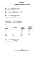
31. 𝑓(𝑥) =

y
2
-4

4

x

a. 𝑓(−1) = −1.  We used the first formula, since −1 is in [−4, 0).
b. 𝑓(0) = 2.  We used the second formula, since 0 is in [0, 4].

c.  𝑓(1) = 2.  We used the second formula, since 1 is in [0, 4].

−1      if  − 4 ≤ 𝑥 ≤ 0
 
{ 𝑥       if 0 < 𝑥 ≤ 4
Technology formula: (-1)*(x<=0)+x*(x>0) (For a graphing calculator, use ≤ instead of <=.)
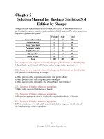
32. 𝑓(𝑥) =

y

-4

4
-1

x

a. 𝑓(−1) = −1.  We used the first formula, since −1 is in [−4, 0].
b. 𝑓(0) = −1.  We used the first formula, since 0 is in [−4, 0].
c. 𝑓(1) = 1.  We used the second formula, since 1 is in (0, 4].

𝑥 2       if  − 2 < 𝑥 ≤ 0
 
{ 1/𝑥       if 0 < 𝑥 ≤ 4
Technology formula: (x^2)*(x<=0)+(1/x)*(033. 𝑓(𝑥) =

Full file at https://./Solution-Manual-for-Applied-Calculus-7th-Edition-by-Waner


Solution Manual for Applied Calculus 7th Edition by Waner

Full file at https://./Solution-Manual-for-Applied-Calculus-7th-Edition-by-Wane
SSoolluuttiioonnss SSeeccttiioonn 1
1..1
1

y

4

-2

0

2

4

x

a. 𝑓(−1) = 1 2 = 1.  We used the first formula, since −1 is in (−2, 0].
b. 𝑓(0) = 0 2 = 0.  We used the first formula, since 0 is in (−2, 0].

c. 𝑓(1) = 1/1 = 1.  We used the second formula, since 1 is in (0, 4].
34. 𝑓(𝑥) =

−𝑥 2       if  − 2 < 𝑥 ≤ 0
 
{ √𝑥      if 0 < 𝑥 < 4

Technology formula: Excel: (-1*x^2)*(x<=0)+SQRT(ABS(x))*(x>0)
TI-83/84 Plus: (-1*x^2)*(x\leq0)+ √(x)*(x>0)

y
2

-2

4

x

-4

a. 𝑓(−1) = −(−1) 2 = −1.  We used the first formula, since −1 is in (−2, 0].
b. 𝑓(0) = −0 2 = 0.  We used the first formula, since 0 is in (−2, 0].

c. 𝑓(1) = √1 = 1.  We used the second formula, since 1 is in (0, 4).

𝑥   
   if  − 1 < 𝑥 ≤ 0
35. 𝑓(𝑥) = 𝑥 + 1      if 0 < 𝑥 ≤ 2  
𝑥   
   if 2 < 𝑥 ≤ 4
Technology formula: x*(x<=0)+(x+1)*(0

Full file at https://./Solution-Manual-for-Applied-Calculus-7th-Edition-by-Waner


Solution Manual for Applied Calculus 7th Edition by Waner

Full file at https://./Solution-Manual-for-Applied-Calculus-7th-Edition-by-Wane
SSoolluuttiioonnss SSeeccttiioonn 1
1..1
1

y
4
2
-1

1

2

4

x

-1

a. 𝑓(0) = 0.  We used the first formula, since 0 is in (−1, 0].

b. 𝑓(1) = 1 + 1 = 2.  We used the second formula, since 1 is in (0, 2].
c. 𝑓(2) = 2 + 1 = 3.  We used the second formula, since 2 is in (0, 2].
d. 𝑓(3) = 3.  We used the third formula, since 3 is in (2, 4].

−𝑥       if  − 1 < 𝑥 < 0
36. 𝑓(𝑥) = 𝑥 − 2      if 0 ≤ 𝑥 ≤ 2  
−𝑥       if 2 < 𝑥 ≤ 4
Technology formula: x*(x<0)+(x-2)*(0<=x)*(x<=2)+(-x)*(2<=.)

y
1
-1

2

4

x

-2
-4

a. 𝑓(0) = 0 − 2 = −2.  We used the second formula, since 0 is in [0, 2].

b. 𝑓(1) = 1 − 2 = −1.  We used the second formula, since 1 is in [0, 2].
c. 𝑓(2) = 2 − 2 = 0.  We used the second formula, since 2 is in [0, 2].
d. 𝑓(3) = −3.  We used the third formula, since 3 is in (2, 4].
37. 𝑓(𝑥) = 𝑥 2 

a. 𝑓(𝑥 + ℎ) = (𝑥 + ℎ) 2  Therefore,

𝑓(𝑥 + ℎ) − 𝑓(𝑥)  = (𝑥 + ℎ) 2 − 𝑥 2

= 𝑥 2 + 2𝑥ℎ + ℎ 2 − 𝑥 2

= 2𝑥ℎ + ℎ 2 = ℎ(2𝑥 + ℎ)

b. Using the answer to part (a),

Full file at https://./Solution-Manual-for-Applied-Calculus-7th-Edition-by-Waner


Solution Manual for Applied Calculus 7th Edition by Waner

Full file at https://./Solution-Manual-for-Applied-Calculus-7th-Edition-by-Wane
        

𝑓(𝑥 + ℎ) − 𝑓(𝑥) ℎ(2𝑥 + ℎ)
=
= 2𝑥 + ℎ 
ℎ
ℎ

SSoolluuttiioonnss SSeeccttiioonn 1
1..1
1

38. 𝑓(𝑥) = 3𝑥 − 1 

a. 𝑓(𝑥 + ℎ) = 3(𝑥 + ℎ) − 1 = 3𝑥 + 3ℎ − 1  Therefore,
𝑓(𝑥 + ℎ) − 𝑓(𝑥)  = 3𝑥 + 3ℎ − 1 − (3𝑥 − 1)

= 3𝑥 + 3ℎ − 1 − 3𝑥 + 1 = 3ℎ

b. Using the answer to part (a),
𝑓(𝑥 + ℎ) − 𝑓(𝑥) 3ℎ
        
=
= 3 
ℎ
ℎ
39. 𝑓(𝑥) = 2 − 𝑥 2 

a. 𝑓(𝑥 + ℎ) = 2 − (𝑥 + ℎ) 2  Therefore,

𝑓(𝑥 + ℎ) − 𝑓(𝑥)  = 2 − (𝑥 + ℎ) 2 − (2 − 𝑥 2)

= 2 − 𝑥 2 − 2𝑥ℎ − ℎ 2 − 2 + 𝑥 2
= −2𝑥ℎ − ℎ 2 = −ℎ(2𝑥 + ℎ)

b. Using the answer to part (a),
𝑓(𝑥 + ℎ) − 𝑓(𝑥) −ℎ(2𝑥 + ℎ)
        
=
= −(2𝑥 + ℎ) 
ℎ
ℎ
40. 𝑓(𝑥) = 𝑥 2 + 𝑥 

a. 𝑓(𝑥 + ℎ) = (𝑥 + ℎ) 2 + (𝑥 + ℎ)  Therefore,

𝑓(𝑥 + ℎ) − 𝑓(𝑥)  = (𝑥 + ℎ) 2 + (𝑥 + ℎ) − (𝑥 2 + 𝑥)

= 𝑥 2 + 2𝑥ℎ + ℎ 2 + 𝑥 + ℎ − 𝑥 2 − 𝑥
= 2𝑥ℎ + ℎ 2 + ℎ = ℎ(2𝑥 + ℎ + 1)

b. Using the answer to part (a),
𝑓(𝑥 + ℎ) − 𝑓(𝑥) ℎ(2𝑥 + ℎ + 1)
        
=
= 2𝑥 + ℎ + 1 
ℎ
ℎ

Applications
41. From the table,
a. 𝑝(2) = 2.95; Pemex produced 2.95 million barrels of crude oil per day in 2010 (𝑡 = 2).
𝑝(3) = 2.94; Pemex produced 2.94 million barrels of crude oil per day in 2011 (𝑡 = 3).

𝑝(6) = 2.79; Pemex produced 2.79 million barrels of crude oil per day in 2014 (𝑡 = 6).

b. 𝑝(4) − 𝑝(2) = 2.91 − 2.95 = −0.04; Crude oil production by Pemex decreased by 0.04 million barrels/day from 2010
(𝑡 = 2) to 2012 (𝑡 = 4).

42. From the table,
a. 𝑠(0) = 2.25; Pemex produced 2.25 million barrels of offshore crude oil per day in 2008 (𝑡 = 0).
𝑠(2) = 1.94; Pemex produced 1.94 million barrels of offshore crude oil per day in 2010 (𝑡 = 2).
𝑠(4) = 1.90; Pemex produced 1.90 million barrels of offshore crude oil per day in 2012 (𝑡 = 4).

Full file at https://./Solution-Manual-for-Applied-Calculus-7th-Edition-by-Waner

Solution Manual for Applied Calculus 7th Edition by Waner

Full file at https://./Solution-Manual-for-Applied-Calculus-7th-Edition-by-Wane
SSoolluuttiioonnss SSeeccttiioonn 1
1..1
1

b. 𝑠(4) − 𝑠(0) = 1.90 − 2.25 = −0.35; Offshore crude oil production by Pemex decreased by 0.35 million barrels/day from
2008 (𝑡 = 0) to 2012 (𝑡 = 4).

43. a. Graph of 𝑝 (below left):

p

p

8

8

7.5

7.5

7

7

6.5

6.5

6

6

5.5

5.5

t

5
0

5
0

t

From the graph, 𝑝(4.5) ≈ 6.5. Interpretation: 𝑡 = 4.5 represents 4.5 years since the start of 2008, or midway through 2012.
Thus, we interpret the answer as follows: The popularity of Twitter midway through 2012 was about 6.5%.
b. The four points suggest a "u"-shaped curve such as a parabola, and only Choice (D) is of this type. (Choice (B) gives an
"upside-down" (concave down) parabola.)
1

2

3

4

5

44. a. Graph of 𝑝 (below left):

p

1

2

2

3

4

5

1

2

3

4

5

p

0.5
0.45
0.4
0.35
0.3
0.25
0.2
0.15
0.1
0.05
0

1

3

4

5

t

0.5
0.45
0.4
0.35
0.3
0.25

0.2
0.15
0.1
0.05
0

t

From the graph, 𝑝(3.5) ≈ 0.075. Interpretation: 𝑡 = 3.5 represents 3.5 years since the start of 2008, or midway through 2011.
Thus, we interpret the answer as follows: The popularity of Delicious midway through 2011 was about 0.075%.
b. Referring to the table of common functions at the end of Section 1.1, we see that the plotted points suggest an exponential
curve that decreases with increaing 𝑡, and only Choice (A) is of this type. (Choice (B) gives an exponential curve that
increases with 𝑡.) Moreover, Choice (A) gives an almost exact fit to the data.

45. From the graph, 𝑓(7) ≈ 1,000.  Because 𝑓   is the number of thousands of housing starts in year 𝑡, we interpret the result
as follows: Approximately 1,000,000 homes were started in 2007.
Similarly, 𝑓(14) ≈ 600:  Approximately 600,000 homes were started in 2014.
Also, we estimate 𝑓(9.5) ≈ 450.  Because 𝑡 = 9.5 is midway between 2009 and 2010, we interpret the result as follows:
450,000 homes were started in the year beginning July 2009.

46. From the graph, 𝑓(3) ≈ 1,500,   𝑓(6) ≈ 1,500,   and 𝑓(8.5) ≈ 500.  Because 𝑓   is the number of thousands of housing
starts in year 𝑡, we interpret the result as follows:

Full file at https://./Solution-Manual-for-Applied-Calculus-7th-Edition-by-Waner


Solution Manual for Applied Calculus 7th Edition by Waner

Full file at https://./Solution-Manual-for-Applied-Calculus-7th-Edition-by-Wane
SSoolluuttiioonnss SSeeccttiioonn 1

1..1
1

𝑓(3) ≈ 1,500:  1.5 million homes were started in 2003.
𝑓(6) ≈ 1,500:  1.5 million homes were started in 2006.

𝑓(8.5) ≈ 500:  500,000 homes were started in the year beginning July 2008.

47. 𝑓(7 − 3) = 𝑓(4) ≈ 1,600  Interpretation: 1,600,000 homes were started in 2004 (𝑡 = 4).

𝑓(7) − 𝑓(3) = 1,000 − 1,500 = −500 
Interpretation:
𝑓(7) − 𝑓(3)  is the change in the number of housing starts (in thousands) from 2003 to 2007; there were 500,000 fewer
housing starts in 2007 than in 2003.
48. 𝑓(13 − 3) = 𝑓(10) ≈ 500  Interpretation: 500,000 homes were started in 2010 (𝑡 = 10).

𝑓(13) − 𝑓(3) = 600 − 1,500 = −900 
Interpretation:
𝑓(13) − 𝑓(3)  is the change in the number of housing starts (in thousands) from 2003 to 2012; there were 900,000 fewer
housing starts in 2012 than in 2003.
49. 𝑓(𝑡 + 5) − 𝑓(𝑡)  measures the change from year 𝑡 to the year five years later. It is greatest when the the line segment from

year 𝑡 to year 𝑡 + 5 is steepest upward-sloping. From the graph, this occurs when 𝑡 = 0, for a change of 1,700 − 1,200 = 500.
Interpretation: The greatest five-year increase in the number of housing starts occurred in 2000–2005.
50. 𝑓(𝑡) − 𝑓(𝑡 − 1)  measures the change from year 𝑡 − 1 to the following year. It is least when the the line segment from year
𝑡 − 1 to year 𝑡 is steepest downward-sloping. From the graph, this occurs when 𝑡 = 7, for a change of 1,000 − 1,500 = −500.
Interpretation: The greatest annual decrease in the number of housing starts occurred in 2006–2007.
51. a. From the graph, 𝑛(2) ≈ 400, 𝑛(4) ≈ 400, 𝑛(4.5) ≈ 350. Because 𝑛(𝑡) is Abercrombie's net income in the year ending
𝑡 + 2004, we interpret the results as follows:
Abercrombie's net income was $400 million in 2006.

Abercrombie's net income was $400 million in 2008.
Abercrombie's net income was $350 million in the year ending June 2009 (because 𝑡 = 4.5 represents June 2009).

b. Increasing most rapidly at 𝑡 ≈ 8 (over the interval [3, 8] the graph is steepest upward-sloping at around 𝑡 = 8.)
Interpretation: Between Dec. 2007 and Dec. 2012 Abercrombie's net income was increasing most rapidly in December 2012.
c. Decreasing most rapidly at 𝑡 ≈ 5 (over the interval [3, 8] the graph is steepest downward-sloping at around 𝑡 = 5.)
Interpretation: Between Dec. 2007 and Dec. 2012, Abercrombie's net income was decreasing most rapidly in Dec. 2009.
52. a. From the graph,
𝑛(0) ≈ 100, 𝑛(4) ≈ 0, 𝑛(5.5) ≈ − 75

Because 𝑛(𝑡) is Pacific Sunwear's net income in the year ending 𝑡 + 2004, we interpret the results as follows:
Pacific Sunwear's net income was $100 million in 2004.
Pacific Sunwear's net income was zero in 2008.
Pacific Sunwear lost $75 million in the year ending June 2010 (𝑡 = 5.5 represents June 2010).

b. Increasing most rapidly at 𝑡 = 9 (the graph is steepest upward-sloping at 𝑡 = 9.) Interpretation: Pacific Sunwear's net
income was increasing most rapidly in 2013.
c. decreasing most rapidly at 𝑡 = 4 (the graph is steepest downward-sloping at 𝑡 = 4.) Interpretation: Pacific Sunwear's net
income was decreasing most rapidly in 2008.

Full file at https://./Solution-Manual-for-Applied-Calculus-7th-Edition-by-Waner


Solution Manual for Applied Calculus 7th Edition by Waner

Full file at https://./Solution-Manual-for-Applied-Calculus-7th-Edition-by-Wane
SSoolluuttiioonnss SSeeccttiioonn 1
1..1
1

53. a. The model is valid for the range 1958 (𝑡 = 0) through 1966 (𝑡 = 8). Thus, an appropriate domain is [0, 8]. 𝑡 ≥ 0 is not an
appropriate domain because it would predict federal funding of NASA beyond 1966, whereas the model is based only on data
up to 1966.
4.5
b. 𝑝(𝑡) =
2
1.07 (𝑡 − 8)
        ⇒         𝑝(5) =

4.5

1.07 (5 − 8)

2

≈ 2.4         Technology formula: 4.5/(1.07^((t-8)^2))

𝑡 = 5 represents 1958 + 5 = 1963, and therefore we interpret the result as follows: In 1963, 2.4% of the U.S. federal budget
was allocated to NASA.
c.  𝑝(𝑡) is increasing most rapidly when the graph is steepest upward-sloping from left to right, and, among the given values of
𝑡, this occurs when 𝑡 = 5. Thus, the percentage of the budget allocated to NASA was increasing most rapidly in 1963.
54. a. [1, 50]; [0, 50] is not an appropriate domain because 𝑝 is undefined at 0.
b. 𝑝(𝑡) = 0.03 +

5
𝑡 0.6

        ⇒         𝑝(40) = 0.03 +

5

≈ 0.58         Technology formula: 0.03+5/t^0.6
40 0.6

𝑡 = 40 represents 1965 + 40 = 2005, and therefore we interpret the result as follows: In 2005, 0.58% of the US federal budget
was allocated to NASA.
c. If we evaluate 𝑝(𝑡) for 𝑡 = 100, 1, 000, 100, 000, 1, 000, 000..., we find values of 𝑝(𝑡) decreasing toward 0.03. Thus, in the
(very) long term, the percentage of the budget allocated to NASA is predicted to approach 0.03%
12, 200
55. 𝑝(𝑡) = 100 1 −
        (𝑡 ≥ 8.5) a. Technology formula: 100*(1-12200/t^4.48)
(
𝑡 4.48 )
b. Graph:

c. Table of values:
𝑡

9

𝑝(𝑡) 35.2

10

11

12

13

14

15

16

17

18

19

20

59.6

73.6

82.2

87.5

91.1

93.4

95.1

96.3

97.1

97.7

98.2

d. From the table, 𝑝(12) = 82.2, so that 82.2% of children are able to speak in at least single words by the age of 12 months.

e. We seek the first value of 𝑡 such that 𝑝(𝑡) is at least 90. Since 𝑡 = 14 has this property (𝑝(14) = 91.1) we conclude that, at 14
months, 90% or more children are able to speak in at least single words.
5.27 × 10 17
        (𝑡 ≥ 30)
)
𝑡 12
a. Technology formula: 100*(1-5.27*10^17/t^12)
56. 𝑝(𝑡) = 100 1 −
(

Full file at https://./Solution-Manual-for-Applied-Calculus-7th-Edition-by-Waner


Solution Manual for Applied Calculus 7th Edition by Waner

Full file at https://./Solution-Manual-for-Applied-Calculus-7th-Edition-by-Wane
SSoolluuttiioonnss SSeeccttiioonn 1
1..1
1

b. Graph:

c. Table of values:

𝑡

𝑝(𝑡)

30

31

32

33

34

35

36

37

38

39

40

0.8

33.1

54.3

68.4

77.9

84.4

88.9

92.0

94.2

95.7

96.9

d. From the table, 𝑝(36) = 88.9, so that 88.9% of children are able to speak in sentences of five or more words by the age of
36 months.

e. We seek the first value of 𝑡 such that 𝑝(𝑡) is at least 75. Since 𝑡 = 34 has this property (𝑝(34) = 77.9) we conclude that, at 34
months, 75% or more children are able to speak in sentences of five or more words.
   if 0 ≤ 𝑡 < 16
8(1.22) 𝑡  
57. 𝑣(𝑡) = 400𝑡 − 6,200      if 16 ≤ 𝑡 < 25
3800  
   if 25 ≤ 𝑡 ≤ 30.

a. 𝑣(10) = 8(1.22) 10 ≈ 58. We used the first formula, since 10 is in [0, 16).

𝑣(16) = 400(16) − 6, 200 = 200. We used the second formula, since 16 is in [16, 25).

𝑣(28) = 3, 800. We used the third formula, since 28 is in [25, 30].
Interpretation: Processor speeds were about 58 MHz in 1990, 200 MHz in 1996, and 3800 MHz in 2008.
b. Technology formula (using 𝑥 as the independent variable):

        (8*(1.22)^x)*(x<16)+(400*x-6200)*(x>=16)*(x<25)+3800*(x>=25)
(For a graphing calculator, use ≤ instead of <=.)
c. Using the above technology formula (for instance, on the Function Evaluator and Grapher on the Web site) we obtain the
graph and table of values. Graph:

Table of values:

Full file at https://./Solution-Manual-for-Applied-Calculus-7th-Edition-by-Waner


Solution Manual for Applied Calculus 7th Edition by Waner

Full file at https://./Solution-Manual-for-Applied-Calculus-7th-Edition-by-Wane
𝑡

𝑣(𝑡)

SSoolluuttiioonnss SSeeccttiioonn 1
1..1
1

0

2

4

6

8

10

12

14

16

8

12

18

26

39

58

87

129

200

18

20

22

24

26

28

30

1,000 1,800 2,600 3,400 3,800 3,800 3,800

d. From either the graph or the table, we see that the speed reached 3,000 MHz around 𝑡 = 23. We can obtain a more precise
answer algebraically by using the formula for the corresponding portion of the graph:
        3, 000 = 400𝑡 − 6, 200
giving
        𝑡 =

9, 200
= 23
400

Since 𝑡 is time since 1980, 𝑡 = 23 corresponds to 2003.
0.12𝑡 2 + 0.04𝑡 + 0.2      if 0 ≤ 𝑡 < 12
58. 𝑣(𝑡) = 1.1(1.22) 𝑡  
   if 12 ≤ 𝑡 < 26
400𝑡 − 10,200  
   if 26 ≤ 𝑡 ≤ 30

a. 𝑣(2) = 0.12(2) 2 + 0.04(2) + 0.2 = 0.76. We used the first formula, since 2 is in [0, 12).
𝑣(12) = 1.1(1.22) 12 ≈ 12. We used the second formula, since 12 is in [12, 26).

𝑣(28) = 400(28) − 10, 200 = 1, 000. We used the third formula, since 28 is in [26, 30].
Interpretation: Processor speeds were about 0.76 MHz in 1972, 12 MHz in 1982, and 1,000 MHz in 1998.
b. Technology formula (using 𝑥 as the independent variable):

(0.12*x^2+0.04*x+0.2)*(x<12)+(1.1*(1.22)^x)*(x>=12)*(x<26)+(400*x-10200)*(x>=26)
(For a graphing calculator, use ≤ instead of <=.)
c. Using the above technology formula (for instance, on the Function Evaluator and Grapher on the Web site) we obtain the
graph and table of values.
Graph:

Table of values:

𝑡

0

𝑣(𝑡) 0.20

2

4

6

8

10

12

14

16

18

20

22

24

26

0.76

2.3

4.8

8.2

13

12

18

26

39

59

87

130

200

28

30

1,000 1,800

d. From either the graph or the table, we see that the speed reached 500 MHz around 𝑡 = 27. We can obtain a more precise
answer algebraically by using the formula for the corresponding portion of the graph:

Full file at https://./Solution-Manual-for-Applied-Calculus-7th-Edition-by-Waner

Solution Manual for Applied Calculus 7th Edition by Waner

Full file at https://./Solution-Manual-for-Applied-Calculus-7th-Edition-by-Wane
        500 = 400𝑡 − 10, 200
giving
        𝑡 =

SSoolluuttiioonnss SSeeccttiioonn 1
1..1
1

10, 700
= 26.75 ≈ 27 to the nearest year
400

Since 𝑡 is time since 1970, 𝑡 = 27 corresponds to 1997.
59. a. Each row of the table gives us a formula with a condition:
First row in words: 10% of the amount over $0 if your income is over $0 and not over $9,225.
Translation to formula:
        0.10𝑥      if 0 < 𝑥 ≤ 9,225.
Second row in words: $922.50 + 15% of the amount over $9,225 if your income is over $9,225 and not over $37,450.
Translation to formula:
        922.50 + 0.15(𝑥 − 9, 225)      if 9,225 < 𝑥 ≤ 37,450.
Continuing in this way leads to the following piecewise-defined function:
0.10𝑥   
   if 0 < 𝑥 ≤ 9,225
922.50 + 0.15(𝑥 − 9,225)  
   if 9,225 < 𝑥 ≤ 37,450

5,156.25 + 0.25(𝑥 − 37,450)  
   if 37,450 < 𝑥 ≤ 90,750
        𝑇 (𝑥) = 18,481.25 + 0.28(𝑥 − 90,750)  
   if 90,750 < 𝑥 ≤ 189,300
46,075.25 + 0.33(𝑥 − 189,300)      if 189,300 < 𝑥 ≤ 411,500
119,401.25 + 0.35(𝑥 − 411,500)      if 411,500 < 𝑥 ≤ 413,200
119,996.25 + 0.396(𝑥 − 413,200)      if 413,200 < 𝑥

b. A taxable income of $45,000 falls in the bracket 37,450 < 𝑥 ≤ 90,750 and so we use the formula
5,156.25 + 0.25(𝑥 − 37,450):

        5,156.25 + 0.25(45,000 − 37,450) = 5,156.25 + 0.25(7,550) = $7,043.75.

60. a. Each row of the table gives us a formula with a condition:
First row in words: 10% of the amount over $0 if your income is over $0 and not over $8,700.
Translation to formula:
        0.10𝑥      if 0 < 𝑥 ≤ 8,700.
Second row in words: $870.00 + 15% of the amount over $8,700 if your income is over $8,700 and not over $35,350.
Translation to formula:
        870.00 + 0.15(𝑥 − 8,700)      if 8,700 < 𝑥 ≤ 35,350.
Continuing in this way leads to the following piecewise-defined function:
0.10𝑥   
   if 0 < 𝑥 ≤ 8,700
870.00 + 0.15(𝑥 − 8,700)  
   if 8,700 < 𝑥 ≤ 35,350
4,867.50 + 0.25(𝑥 − 35,350)  
   if 35,350 < 𝑥 ≤ 85,650
        𝑇 (𝑥) =
17,442.50 + 0.28(𝑥 − 85,650)      if 85,650 < 𝑥 ≤ 178,650
43,482.50 + 0.33(𝑥 − 178,650)      if 178,650 < 𝑥 ≤ 388,350

112,683.50 + 0.35(𝑥 − 388,350)      if 388,350 < 𝑥

b. A taxable income of $45,000 falls in the bracket 35,350 < 𝑥 ≤ 85,650 and so we use the formula
4,867.50 + 0.25(𝑥 − 35,350):

        4,867.50 + 0.25(45,000 − 35,350) = 4,867.50 + 0.25(9,650) = $7,280.00.

Full file at https://./Solution-Manual-for-Applied-Calculus-7th-Edition-by-Waner


Solution Manual for Applied Calculus 7th Edition by Waner

Full file at https://./Solution-Manual-for-Applied-Calculus-7th-Edition-by-Wane
SSoolluuttiioonnss SSeeccttiioonn 1
1..1
1

Communication and reasoning exercises

61. The dependent variable is a function of the independent variable. Here, the market price of gold 𝑚 is a function of time 𝑡.
Thus, the independent variable is 𝑡 and the dependent variable is 𝑚.

62. The dependent variable is a function of the independent variable. Here, the weekly profit 𝑃 is a function of the selling
price 𝑠. Thus, the independent variable is 𝑠 and the dependent variable is 𝑃 .

63. To obtain the function notation, write the dependent variable as a function of the independent variable. Thus 𝑦 = 4𝑥 2 − 2
can be written as
        𝑓(𝑥) = 4𝑥 2 − 2  or 𝑦(𝑥) = 4𝑥 2 − 2
𝐶(𝑡) = −0.34𝑡 2 + 0.1𝑡 can be written as

64. To obtain the equation notation, introduce a dependent variable instead of the function notation. Thus
        𝑐 = −0.34𝑡 2 + 0.1𝑡 or 𝑦 = −0.34𝑡 2 + 0.1𝑡
65. False. A graph usually gives infinitely many values of the function while a numerical table will give only a finite number
of values.
66. True. An algebraically specified function 𝑓   is specified by algebraic formulas for 𝑓(𝑥).  Given such formulas, we can
construct the graph of 𝑓   by plotting the points (𝑥, 𝑓(𝑥))  for values of 𝑥 in the domain of 𝑓. 

67. False. In a numerically specified function, only certain values of the function are specified so we cannot know its value on
every real number in [0, 10], whereas an algebraically specified function would give values for every real number in [0, 10].
68. False. A graphically specified function is specified by a graph. However, we cannot always expect to find an algebraic
formula whose graph is exactly the graph that is given.
69. Functions with infinitely many points in their domain (such as 𝑓(𝑥) = 𝑥 2  ) cannot be specified numerically. So, the
assertion is false.
70. A numerical model supplies only the values of a function at specific values of the independent variable, whereas an
algebraic model supplies the value of a function at every point in its domain. Thus, an algebraic model supplies more
information.
71. As the text reminds us: to evaluate 𝑓   of a quantity (such as 𝑥 + ℎ) replace 𝑥 everywhere by the whole quantity 𝑥 + ℎ:
𝑓(𝑥) 

= 𝑥2 − 1

𝑓(𝑥 + ℎ)  = (𝑥 + ℎ) 2 − 1.

72. Knowing 𝑓(𝑥)  for two values of 𝑥 does not convey any information about 𝑓(𝑥)  at any other value of 𝑥. Interpolation is
only a way of estimating 𝑓(𝑥)  at values of 𝑥 not given.

73. If two functions are specified by the same formula 𝑓(𝑥),   say, their graphs must follow the same curve 𝑦 = 𝑓(𝑥). 
However, it is the domain of the function that specifies what portion of the curve appears on the graph. Thus, if the functions
have different domains, their graphs will be different portions of the curve 𝑦 = 𝑓(𝑥). 

Full file at https://./Solution-Manual-for-Applied-Calculus-7th-Edition-by-Waner


Solution Manual for Applied Calculus 7th Edition by Waner

Full file at https://./Solution-Manual-for-Applied-Calculus-7th-Edition-by-Wane
SSoolluuttiioonnss SSeeccttiioonn 1
1..1
1

74. If we plot points of the graphs 𝑦 = 𝑓(𝑥)  and 𝑦 = 𝑔(𝑥), we see that, since 𝑔(𝑥) = 𝑓(𝑥) + 10,   we must add 10 to the 𝑦

-coordinate of each point in the graph of 𝑓   to get a point on the graph of 𝑔. Thus, the graph of 𝑔 is 10 units higher up than the
graph of 𝑓. 

75. Suppose we already have the graph of 𝑓   and want to construct the graph of 𝑔. We can plot a point of the graph of 𝑔 as
follows: Choose a value for 𝑥 (𝑥 = 7, say) and then "look back" 5 units to read off 𝑓(𝑥 − 5)  (𝑓(2)  in this instance). This

value gives the 𝑦-coordinate we want. In other words, points on the graph of 𝑔 are obtained by "looking back 5 units" to the
graph of 𝑓   and then copying that portion of the curve. Put another way, the graph of 𝑔 is the same as the graph of 𝑓,   but
shifted 5 units to the right:

76. Suppose we already have the graph of 𝑓   and want to construct the graph of 𝑔. We can plot a point of the graph of 𝑔 as
follows: Choose a value for 𝑥 (𝑥 = 7, say) and then look on the other side of the 𝑦-axis to read off 𝑓(−𝑥)  (𝑓(−7)  in this

instance). This value gives the 𝑦-coordinate we want. In other words, points on the graph of 𝑔 are obtained by "looking back"
to the graph of 𝑓   on the opposite side of the 𝑦-axis and then copying that portion of the curve. Put another way, the graph of
𝑔(𝑥) is the mirror image of the graph of 𝑓(𝑥)  in the 𝑦-axis:

Full file at https://./Solution-Manual-for-Applied-Calculus-7th-Edition-by-Waner

Solution Manual for Applied Calculus 7th Edition by Waner

Full file at https://./Solution-Manual-for-Applied-Calculus-7th-Edition-by-Wane
SSoolluuttiioonnss SSeeccttiioonn 1
1..2
2
SSeeccttiioonn 1
1..2
2

1. 𝑓(𝑥) = 𝑥 2 + 1  with domain (−∞, +∞)
𝑔(𝑥) = 𝑥 − 1 with domain (−∞, +∞)

a. 𝑠(𝑥) = 𝑓(𝑥) + 𝑔(𝑥) = (𝑥 2 + 1) + (𝑥 − 1) = 𝑥 2 + 𝑥 

b. Since both functions are defined for every real number 𝑥, the domain of 𝑠 is the set of all real numbers: (−∞, +∞).
c. 𝑠(−3) = (−3) 2 + (−3) = 9 − 3 = 6

2. 𝑓(𝑥) = 𝑥 2 + 1  with domain (−∞, +∞)
𝑔(𝑥) = 𝑥 − 1 with domain (−∞, +∞)

a. 𝑑(𝑥) = 𝑔(𝑥) − 𝑓(𝑥) = (𝑥 − 1) − (𝑥 2 + 1) = −𝑥 2 + 𝑥 − 2 

b. Since both functions are defined for every real number 𝑥, the domain of 𝑑 is the set of all real numbers: (−∞, +∞).
c. 𝑑(−1) = −(−1) 2 + (−1) − 2 = −4

3. 𝑔(𝑥) = 𝑥 − 1 with domain (−∞, +∞)
𝑢(𝑥) = √𝑥 + 10 with domain [−10, 0)

a. 𝑝(𝑥) = 𝑔(𝑥)𝑢(𝑥) = (𝑥 − 1)√𝑥 + 10

b. The domain of 𝑝 consists of all real numbers 𝑥 simultaneously in the domains of 𝑔 and 𝑢; that is, [−10, 0).
c. 𝑝(−6) = (−6 − 1)√−6 + 10 = (−7)(2) = −14
4. ℎ(𝑥) = 𝑥 + 4 with domain [10, +∞)
𝑣(𝑥) = √10 − 𝑥 with domain [0, 10]

a. 𝑝(𝑥) = ℎ(𝑥)𝑣(𝑥) = (𝑥 + 4)√10 − 𝑥

b. The domain of 𝑝 consists of all real numbers 𝑥 simultaneously in the domains of ℎ and 𝑣; that is, the single point
𝑥 = 10.

c. As 1 is not in the domain of 𝑝, 𝑝(1) is not defined.
5. 𝑔(𝑥) = 𝑥 − 1 with domain (−∞, +∞)
𝑣(𝑥) = √10 − 𝑥 with domain [0, 10]
a. 𝑞(𝑥) =

𝑣(𝑥)
𝑔(𝑥)

=

√10 − 𝑥

𝑥−1

b. The domain of 𝑞 consists of all real numbers 𝑥 simultaneously in the domains of 𝑣 and 𝑔 such that 𝑔(𝑥) ≠ 0. Since
        𝑔(𝑥) = 0 when 𝑥 − 1 = 0, or 𝑥 = 1

we exclude 𝑥 = 1 from the domain of the quotient. Thus, the domain consists of all 𝑥 in [0, 10] excluding 𝑥 = 1 (since

𝑔(1) = 0), or 0 ≤ 𝑥 ≤ 10; 𝑥 ≠ 1.

c. As 1 is not in the domain of 𝑞, 𝑞(1) is not defined.
6. 𝑔(𝑥) = 𝑥 − 1 with domain (−∞, +∞)
𝑣(𝑥) = √10 − 𝑥 with domain [0, 10]

Full file at https://./Solution-Manual-for-Applied-Calculus-7th-Edition-by-Waner


Solution Manual for Applied Calculus 7th Edition by Waner

Full file at https://./Solution-Manual-for-Applied-Calculus-7th-Edition-by-Wane
a. 𝑞(𝑥) =

𝑔(𝑥)

𝑣(𝑥)

=

SSoolluuttiioonnss SSeeccttiioonn 1
1..2
2

𝑥−1

√10 − 𝑥

b. The domain of 𝑞 consists of all real numbers 𝑥 simultaneously in the domains of 𝑣 and 𝑔 such that 𝑣(𝑥) ≠ 0. Since
        𝑣(𝑥) = 0 when √10 − 𝑥 = 0, or 𝑥 = 10

we exclude 𝑥 = 10 from the domain of the quotient. Thus, the domain consists of all 𝑥 in [0, 10] excluding 𝑥 = 10;
that is, [0, 10).

c. 1 is in the domain of 𝑞, and 𝑞(1) =

1−1

√10 − 1

=0

7. 𝑓(𝑥) = 𝑥 2 + 1  with domain (−∞, +∞)
a. 𝑚(𝑥) = 5𝑓(𝑥) = 5(𝑥 2 + 1) 

b. The domain of 𝑚 is the same as the domain of 𝑓:  (−∞, +∞).
c. 𝑚(1) = 5𝑓(1) = 5(1 2 + 1) = 10 

8. 𝑢(𝑥) = √𝑥 + 10 with domain [−10, 0)
a. 𝑚(𝑥) = 3𝑢(𝑥) = 3√𝑥 + 10

b. The domain of 𝑚 is the same as the domain of 𝑢: [−10, 0)
c. 𝑚(−1) = 3𝑢(−1) = 3√−1 + 10 = 9

Applications

9. Number of music files = Starting number + New files = 200 + 10 × Number of days
So, 𝑁(𝑡) = 200 + 10𝑡 (𝑁 = number of music files, 𝑡 = time in days)

10. Free space left = Current amount − Decrease = 50 − 5 × Number of months

So, 𝑆(𝑡) = 50 − 5𝑡 (𝑆 = space on your HD, 𝑡 = time in months)
11. Take 𝑦 to be the width. Since the length is twice the width,
        𝑥 = 2𝑦, so 𝑦 = 𝑥/2.
The area is therefore

        𝐴(𝑥) = 𝑥𝑦 = 𝑥(𝑥/2) = 𝑥 2/2.

12. Take 𝑦 to be the length, so the perimeter is 𝑥 + 𝑦 + 𝑥 + 𝑦 = 2(𝑥 + 𝑦)
The area is 100 sq. ft., so
100
        100 = 𝑥𝑦, giving 𝑦 =
𝑥
Thus, the perimeter is
        𝑃 (𝑥) = 2(𝑥 + 𝑦) = 2(𝑥 + 100/𝑥) or 2𝑥 + 200/𝑥

13. Since the patch is square the width and length are both equal to 𝑥. The costs are:
        East and West sides: 4𝑥 + 4𝑥 = 8𝑥

        North and South Sides: 2𝑥 + 2𝑥 = 4𝑥

Full file at https://./Solution-Manual-for-Applied-Calculus-7th-Edition-by-Waner


Solution Manual for Applied Calculus 7th Edition by Waner

Full file at https://./Solution-Manual-for-Applied-Calculus-7th-Edition-by-Wane
        Total cost 𝐶(𝑥) = 8𝑥 + 4𝑥 = 12𝑥

SSoolluuttiioonnss SSeeccttiioonn 1
1..2

2

14. Since the garden is square the width and length are both equal to 𝑥. The costs are:
        East and West sides: 2𝑥 + 2𝑥 = 4𝑥
        South Side: 4𝑥

        Total cost 𝐶(𝑥) = 4𝑥 + 4𝑥 = 8𝑥

15. The number of hours you study, ℎ(𝑛), equals 4 on Sunday through Thursday and equals 0 on the remaining days.
Since Sunday corresponds to 𝑛 = 1 and Thursday to 𝑛 = 5, we get
        ℎ(𝑛) =

4      if 1 ≤ 𝑛 ≤ 5
.
{ 0      if 𝑛 > 5

16. The number of hours you watch movies, ℎ(𝑛), equals 5 on Saturday (𝑛 = 7) and Sunday (𝑛 = 1) and equals 2 on
the remaining days.
5      if 𝑛 = 1 or 𝑛 = 7
        ℎ(𝑛) =
.
{ 2      otherwise 
17. For a linear cost function, 𝐶(𝑥) = 𝑚𝑥 + 𝑏. Here, 𝑚 = marginal cost = $1,500 per piano, 𝑏 = fixed cost = $1,000.
Thus, the daily cost function is
        𝐶(𝑥) = 1,500𝑥 + 1,000.
a. The cost of manufacturing 3 pianos is
        𝐶(3) = 1,500(3) + 1,000 = 4,500 + 1,000 = $5,500.
b. The cost of manufacturing each additional piano (such as the third one or the 11th one) is the marginal cost,
𝑚 = $1,500.
c. Same answer as (b).

d. Variable cost = part of the cost function that depends on 𝑥 = $1,500𝑥
Fixed cost = constant summand of the cost function = $1,000
Marginal cost = slope of the cost function = $1,500 per piano
e. Graph:
C
8,000
7,000
6,000
5,000
4,000
3,000
2,000
1,000

x
0

1

2

3

4

18. For a linear cost function, 𝐶(𝑥) = 𝑚𝑥 + 𝑏. Here, 𝑚 = marginal cost = $88 per tuxedo, 𝑏 = fixed cost = $20.
Thus, the cost function is
        𝐶(𝑥) = 88𝑥 + 20.
a. The cost of renting 2 tuxes is
        𝐶(2) = 88(2) + 20 = $196

b. The cost of each additional tux is the marginal cost 𝑚 = $88.

Full file at https://./Solution-Manual-for-Applied-Calculus-7th-Edition-by-Waner


Solution Manual for Applied Calculus 7th Edition by Waner

Full file at https://./Solution-Manual-for-Applied-Calculus-7th-Edition-by-Wane
SSoolluuttiioonnss SSeeccttiioonn 1
1..2
2

c. Same answer as (b).
d. Variable cost = part of the cost function that depends on 𝑥 = $88𝑥
Fixed cost = constant summand of the cost function = $20
Marginal cost = slope of the cost function = $88 per tuxedo
e. Graph:
C
400
350
300
250
200
150
100
50
0

1

2

3

4

x

19. a. For a linear cost function, 𝐶(𝑥) = 𝑚𝑥 + 𝑏. Here, 𝑚 = marginal cost = $0.40 per copy, 𝑏 = fixed cost = $70.
Thus, the cost function is 𝐶(𝑥) = 0.4𝑥 + 70.

The revenue function is 𝑅(𝑥) = 0.50𝑥. (𝑥 copies at 50¢ per copy)
The profit function is
𝑃 (𝑥) = 𝑅(𝑥) − 𝐶(𝑥)

= 0.5𝑥 − (0.4𝑥 + 70)
= 0.5𝑥 − 0.4𝑥 − 70
= 0.1𝑥 − 70

b. 𝑃 (500) = 0.1(500) − 70 = 50 − 70 = −20

Since 𝑃 is negative, this represents a loss of $20.
c. For breakeven, 𝑃 (𝑥) = 0:
        0.1𝑥 − 70 = 0
        0.1𝑥 = 70
        𝑥 =

70
= 700 copies
0.1

20. a. For a linear cost function, 𝐶(𝑥) = 𝑚𝑥 + 𝑏. Here, 𝑚 = marginal cost = $0.15 per serving, 𝑏 = fixed cost = $350.
Thus, the cost function is 𝐶(𝑥) = 0.15𝑥 + 350.
The revenue function is 𝑅(𝑥) = 0.50𝑥.
The profit function is
𝑃 (𝑥) = 𝑅(𝑥) − 𝐶(𝑥)

= 0.50𝑥 − (0.15𝑥 + 350)
= 0.35𝑥 − 350

b. For break-even, 𝑃 (𝑥) = 0:
        0.35𝑥 − 350 = 0
        0.35𝑥 = 350

        𝑥 = 1,000 servings

Full file at https://./Solution-Manual-for-Applied-Calculus-7th-Edition-by-Waner


Solution Manual for Applied Calculus 7th Edition by Waner

Full file at https://./Solution-Manual-for-Applied-Calculus-7th-Edition-by-Wane
SSoolluuttiioonnss SSeeccttiioonn 1
1..2
2

c.  𝑃 (1,500) = 0.35(1,500) − 350 = 525 − 350 = $175, representing a profit of $175.
21. The revenue per jersey is $100. Therefore, Revenue 𝑅(𝑥) = $100𝑥.
Profit = Revenue − Cost
𝑃 (𝑥) = 𝑅(𝑥) − 𝐶(𝑥)

= 100𝑥 − (2,000 + 10𝑥 + 0.2𝑥 2)
= −2,000 + 90𝑥 − 0.2𝑥 2

To break even, 𝑃 (𝑥) = 0, so −2,000 + 90𝑥 − 0.2𝑥 2 = 0.

This is a quadratic equation with 𝑎 = −0.2, 𝑏 = 90, 𝑐 = −2,000 and solution
𝑥=
=

−𝑏 ± √𝑏 2 − 4𝑎𝑐
2𝑎

−90 ± √(90) 2 − 4(−2,000)(−0.2)
2(−0.2)

≈ 23.44 or 426.56 jerseys.

Since the second value is outside the domain, we use the first: 𝑥 = 23.44 jerseys. To make a profit, 𝑥 should be larger
than this value: at least 24 jerseys.
22. The revenue per pair is $120. Therefore, Revenue 𝑅(𝑥) = $120𝑥.
Profit = Revenue − Cost
𝑃 (𝑥) = 𝑅(𝑥) − 𝐶(𝑥)

= 120𝑥 − (3,000 + 8𝑥 + 0.1𝑥 2)
= −3,000 + 112 − 0.1𝑥 2

To break even, 𝑃 (𝑥) = 0, so −3,000 + 112 − 0.1𝑥 2 = 0.

This is a quadratic equation with 𝑎 = −0.1, 𝑏 = 112, 𝑐 = −3,000 and solution

𝑥=

−𝑏 ± √𝑏 2 − 4𝑎𝑐
2𝑎

=

−90 ± √(112) 2 − 4(−3,000)(−0.1)
2(−0.1)

≈ 27.46 or 1092.54 jerseys.

Since the second value is outside the domain, we use the first: 𝑥 = 27.46 jerseys. To make a profit, 𝑥 should be larger
than this value: at least 28 pairs of cleats.
23. The revenue from one thousand square feet (𝑥 = 1) is $0.1 million. Therefore, Revenue 𝑅(𝑥) = $0.1𝑥. Profit =
Revenue − Cost
𝑃 (𝑥) = 𝑅(𝑥) − 𝐶(𝑥)

= 0.1𝑥 − (1.7 + 0.12𝑥 − 0.0001𝑥 2)
= −1.7 − 0.02𝑥 + 0.0001𝑥 2

To break even, 𝑃 (𝑥) = 0, so −1.7 − 0.02𝑥 + 0.0001𝑥 2 = 0.

This is a quadratic equation with 𝑎 = 0.0001, 𝑏 = −0.02, 𝑐 = −1.7 and solution

Full file at https://./Solution-Manual-for-Applied-Calculus-7th-Edition-by-Waner


Solution Manual for Applied Calculus 7th Edition by Waner

Full file at https://./Solution-Manual-for-Applied-Calculus-7th-Edition-by-Wane
SSoolluuttiioonnss SSeeccttiioonn 1
1..2
2

𝑥=
=

−𝑏 ± √𝑏 2 − 4𝑎𝑐
2𝑎

0.02 ± √(−0.02) 2 − 4(0.0001)(−1.7)
2(0.0001)

=

0.02 ± 0.03286
≈ 264 thousand square feet
0.0002

24. The revenue from one thousand square feet (𝑥 = 1) is $0.2 million. Therefore, Revenue 𝑅(𝑥) = $0.2𝑥.
Profit = Revenue − Cost
𝑃 (𝑥) = 𝑅(𝑥) − 𝐶(𝑥)

= 0.2𝑥 − (1.7 + 0.14𝑥 − 0.0001𝑥 2)
= −1.7 + 0.06𝑥 + 0.0001𝑥 2

To break even, 𝑃 (𝑥) = 0, so −1.7 + 0.06𝑥 + 0.0001𝑥 2 = 0.

This is a quadratic equation with 𝑎 = 0.0001, 𝑏 = 0.06, 𝑐 = −1.7 and solution

𝑥=
=

−𝑏 ± √𝑏 2 − 4𝑎𝑐
2𝑎

−0.06 ± √(−0.06) 2 − 4(0.0001)(−1.7)
2(0.0001)

=

−0.06 ± 0.0654
≈ 27 thousand square feet
0.0002

25. The hourly profit function is given by
        Profit = Revenue − Cost
        𝑃 (𝑥) = 𝑅(𝑥) − 𝐶(𝑥)
(Hourly) cost function: This is a fixed cost of $5,132 only:
        𝐶(𝑥) = 5,132
(Hourly) revenue function: This is a variable of $100 per passenger cost only:
        𝑅(𝑥) = 100𝑥
Thus, the profit function is
        𝑃 (𝑥) = 𝑅(𝑥) − 𝐶(𝑥)
        𝑃 (𝑥) = 100𝑥 − 5,132

For the domain of 𝑃 (𝑥), the number of passengers 𝑥 cannot exceed the capacity: 405. Also, 𝑥 cannot be negative.
Thus, the domain is given by 0 ≤ 𝑥 ≤ 405, or [0, 405].
        For breakeven, 𝑃 (𝑥) = 0
        100𝑥 − 5,132 = 0

        100𝑥 = 5,132, or 𝑥 =

5,132
= 51.32
100

If 𝑥 is larger than this, then the profit function is positive, and so there should be at least 52 passengers (note that 𝑥
must be a whole number); 𝑥 ≥ 52, for a profit.

26. The hourly profit function is given by
        Profit = Revenue − Cost
        𝑃 (𝑥) = 𝑅(𝑥) − 𝐶(𝑥)
(Hourly) cost function: This is a fixed cost of $3,885 only:
        𝐶(𝑥) = 3,885

Full file at https://./Solution-Manual-for-Applied-Calculus-7th-Edition-by-Waner


Solution Manual for Applied Calculus 7th Edition by Waner

Full file at https://./Solution-Manual-for-Applied-Calculus-7th-Edition-by-Wane
SSoolluuttiioonnss SSeeccttiioonn 1
1..2
2

(Hourly) revenue function: This is a variable of $100 per passenger cost only:
        𝑅(𝑥) = 100𝑥
Thus, the profit function is
        𝑃 (𝑥) = 𝑅(𝑥) − 𝐶(𝑥)

        𝑃 (𝑥) = 100𝑥 − 3,885

For the domain of 𝑃 (𝑥), the number of passengers 𝑥 cannot exceed the capacity: 295. Also, 𝑥 cannot be negative.
Thus, the domain is given by 0 ≤ 𝑥 ≤ 295, or [0, 295].
        For breakeven, 𝑃 (𝑥) = 0
        100𝑥 − 3,885 = 0

        100𝑥 = 3,885, or 𝑥 =

3,885
= 38.85
100

If 𝑥 is larger than this, then the profit function is positive, and so there should be at least 39 passengers (note that 𝑥
must be a whole number); 𝑥 ≥ 39, for a profit.

27. To compute the break-even point, we use the profit function: Profit = Revenue − Cost
        𝑃 (𝑥) = 𝑅(𝑥) − 𝐶(𝑥)
        𝑅(𝑥) = 2𝑥         $2 per unit

                 = 40% of Revenue + 6,000 = 0.4(2𝑥) + 6,000 = 0.8𝑥 + 6,000
        𝐶(𝑥) = Variable Cost + Fixed Cost
Thus, 𝑃 (𝑥) = 𝑅(𝑥) − 𝐶(𝑥)

        𝑃 (𝑥) = 2𝑥 − (0.8𝑥 + 6,000) = 1.2𝑥 − 6,000
For breakeven, 𝑃 (𝑥) = 0
        1.2𝑥 − 6,000 = 0

6,000
= 5,000

1.2𝑥
Therefore, 5,000 units should be made to break even.
        1.2𝑥 = 6,000, so 𝑥 =

28. To compute the break-even point, we use the profit function: Profit = Revenue − Cost
        𝑃 (𝑥) = 𝑅(𝑥) − 𝐶(𝑥) n         𝑅(𝑥) = 5𝑥         $5 per unit
                 = 30% of Revenue + 7,000 = 0.3(5𝑥) + 7,000 = 1.5𝑥 + 7,000
        𝐶(𝑥) = Variable Cost + Fixed Cost
Thus, 𝑃 (𝑥) = 𝑅(𝑥) − 𝐶(𝑥)

        𝑃 (𝑥) = 5𝑥 − (1.5𝑥 + 7,000) = 3.5𝑥 − 7,000
For breakeven, 𝑃 (𝑥) = 0

        3.5𝑥 = 7,000, so 𝑥 = 2,000 units.

29. To compute the break-even point, we use the revenue and cost functions:
        𝑅(𝑥) = Selling price × Number of units = 𝑆𝑃 𝑥
        𝐶(𝑥) = Variable Cost + Fixed Cost = 𝑉 𝐶𝑥 + 𝐹 𝐶
(Note that "variable cost per unit" is marginal cost.) For breakeven
        𝑅(𝑥) = 𝐶(𝑥)
        𝑆𝑃 𝑥 = 𝑉 𝐶𝑥 + 𝐹 𝐶
Solve for 𝑥:

Full file at https://./Solution-Manual-for-Applied-Calculus-7th-Edition-by-Waner


Solution Manual for Applied Calculus 7th Edition by Waner

Full file at https://./Solution-Manual-for-Applied-Calculus-7th-Edition-by-Wane
SSoolluuttiioonnss SSeeccttiioonn 1

1..2
2

        𝑆𝑃 𝑥 − 𝑉 𝐶𝑥 = 𝐹 𝐶 n         𝑥(𝑆𝑃 − 𝑉 𝐶) = 𝐹 𝐶, so 𝑥 =

𝐹𝐶
.
𝑆𝑃 − 𝑉 𝐶

30. To compute the break-even point, we use the revenue and cost functions:
        𝑅(𝑥) = 𝑆𝑃 𝑥;𝐶(𝑥) = 𝑉 𝐶𝑥 + 𝐹 𝐶
At breakeven
        𝑅(𝐵𝐸) = 𝐶(𝐵𝐸)
        𝑆𝑃 (𝐵𝐸) = 𝑉 𝐶(𝐵𝐸) + 𝐹 𝐶

Thus, 𝐹 𝐶 = 𝑆𝑃 (𝐵𝐸) − 𝑉 𝐶(𝐵𝐸) = 𝐵𝐸(𝑆𝑃 − 𝑉 𝐶).

31. Take 𝑥 to be the number of grams of perfume he buys and sells. The profit function is given by Profit = Revenue −
Cost: that is, 𝑃 (𝑥) = 𝑅(𝑥) − 𝐶(𝑥)
Cost function 𝐶(𝑥):
Fixed costs:

Cheap perfume @ $20 per g:

20𝑥

20,000

Transportation @ $30 per 100 g: 0.3𝑥

Thus the cost function is
        𝐶(𝑥) = 20𝑥 + 0.3𝑥 + 20,000 = 20.3𝑥 + 20,000
Revenue function R(x)
        𝑅(𝑥) = 600𝑥         $600 per gram
Thus, the profit function is
        𝑃 (𝑥) = 𝑅(𝑥) − 𝐶(𝑥)

        𝑃 (𝑥) = 600𝑥 − (20.3𝑥 + 20,000) = 579.7𝑥 − 20,000, with domain 𝑥 ≥ 0.
For breakeven, 𝑃 (𝑥) = 0

        579.7𝑥 − 20,000 = 0

20,000
≈ 34.50
579.7
Thus, he should buy and sell 34.50 grams of perfume per day to break even.
        579.7𝑥 = 20,000, so 𝑥 =

32. Take 𝑥 to be the number of grams of perfume he buys and sells. The profit function is given by
        Profit = Revenue − Cost
Cost function: 𝐶(𝑥) = 400𝑥 + 30𝑥 = 430𝑥
Revenue: 𝑅(𝑥) = 420𝑥

Thus, the profit function is 𝑃 (𝑥) = 𝑅(𝑥) − 𝐶(𝑥) = 420𝑥 − 430𝑥 = −10𝑥, with domain 𝑥 ≥ 0.
For breakeven, −10𝑥 = 0, so 𝑥 = 0 grams per day; he should shut down the operation.
33. a. To graph the demand function we use technology with the formula
        760/x-1
and with xMin = 60 and xMax = 400.

Full file at https://./Solution-Manual-for-Applied-Calculus-7th-Edition-by-Waner