MC và các hệ thống phổ Bá P4

4
Implementation Issues
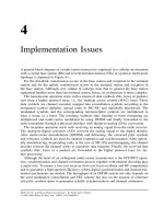
A general block diagram of a multi-carrier transceiver employed in a cellular environment
with a central base station (BS) and several terminal stations (TSs) in a point to multi-point
topology is depicted in Figure 4-1.
For the downlink, transmission occurs in the base station and reception in the terminal
station and for the uplink, transmission occurs in the terminal station and reception in
the base station. Although very similar in concept, note that in general the base station
equipment handles more than one terminal station, hence, its architecture is more complex.
The transmission operation starts with a stream of data symbols (bits, bytes or packets)
sent from a higher protocol layer, i.e., the medium access control (MAC) layer. These
data symbols are channel encoded, mapped into constellation symbols according to the
designated symbol alphabet, spread (only in MC-SS) and optionally interleaved. The
modulated symbols and the corresponding reference/pilot symbols are multiplexed to
form a frame or a burst. The resulting symbols after framing or burst formatting are
multiplexed and multi-carrier modulated by using OFDM and finally forwarded to the
radio transmitter through a physical interface with digital-to-analog (D/A) conversion.
The reception operation starts with receiving an analog signal from the radio receiver.
The analog-to-digital converter (A/D) converts the analog signal to the digital domain.
After multi-carrier demodulation (IOFDM) and deframing, the extracted pilot symbols
and reference symbols are used for channel estimation and synchronization. After option-
ally deinterleaving, despreading (only in the case of MC-SS) and demapping, the channel
decoder corrects the channel errors to guarantee data integrity. Finally, the received data
symbols (bits, bytes or a packet) are forwarded to the higher protocol layer for fur-
ther processing.
Although the heart of an orthogonal multi-carrier transmission is the FFT/IFFT opera-
tion, synchronization and channel estimation process together with channel decoding play
a major role. To ensure a low-cost receiver (low-cost local oscillator and RF components)
and to guarantee a high spectral efficiency, robust digital synchronization and channel esti-
mation mechanisms are needed. The throughput of an OFDM system not only depends on
the used modulation constellation and FEC scheme but also on the amount of reference

and pilot symbols spent to guarantee reliable synchronization and channel estimation.
Multi-Carrier and Spread Spectrum Systems K. Fazel and S. Kaiser

2003 John Wiley & Sons, Ltd ISBN: 0-470-84899-5
116 Implementation Issues
Spreader
(only for
MC-SS)
Interleaver
& Mapper
OFDM
D/A
Analog
front end
Channel
decoder
Despreader
(only for
MC-SS)
Demapper
& Deinterl.
IOFDM
A/D
Analog
front end
Deframing
Framing
Channel
estimation
Digital

VCO
Channel
Transmitter, Tx
Receiver, Rx
AGC
Channel state information (CSI)
Window
Sampling rate
Tx
data
Rx
data
Channel
encoder
Frequency and time
synchronization
Figure 4-1 General block diagram of a multi-carrier transceiver
In Chapter 2 the different despreading and detection strategies for MC-SS systems were
analysed. It was shown that with an appropriate detection strategy, especially in full load
conditions (where all users are active) a high system capacity can be achieved. In the
performance analysis in Chapter 2 we assumed that the modem is perfectly synchronized
and the channel is perfectly known at the receiver.
The principal goal of this chapter is to describe in detail the remaining components
of a multi-carrier transmission scheme with or without spreading. The focus is given
to multi-carrier modulation/demodulation, digital I/Q generation, sampling, channel cod-
ing/decoding, framing/deframing, synchronization, and channel estimation mechanisms.
Especially for synchronization and channel estimation units the effects of the transceiver
imperfections (i.e., frequency drift, imperfect sampling time, phase noise) are highlighted.
Finally, the effects of the amplifier non-linearity in multi-carrier transmission are analyzed.
4.1 Multi-Carrier Modulation and Demodulation

After symbol mapping (e.g., M-QAM) and spreading (in MC-SS), each block of N
c
complex-valued symbols is serial-to-parallel (S/P) converted and submitted to the multi-
carrier modulator, where the symbols are transmitted simultaneously on N
c
parallel sub-
carriers, each occupying a small fraction (1/N
c
) of the total available bandwidth B.
Figure 4-2 shows the block diagram of a multi-carrier transmitter. The transmitted
baseband signal is given by
s(t) =
1
N
c
+∞

i=−∞
N
c
−1

n=0
d
n,i
g(t − iT
s
) e
j 2πf
n

t
,(4.1)
Multi-Carrier Modulation and Demodulation 117
Mapping
S
/
P
Pulse
shaping g(t)
Pulse
shaping g(t)
Pulse
shaping g(t)
+
exp(j2pf
0
t)
exp(j2pf
1
t)
exp(j2pf
Nc −1
t)
s(t)
.
.
.
exp(j2pf
c
t)

s
RF
(t)
Figure 4-2 Block diagram of a multi-carrier transmitter
where N
c
is the number of sub-carriers, 1/T
s
is the symbol rate associated with each
sub-carrier, g(t) is the impulse response of the transmitter filters, d
n,i
is the complex
constellation symbol, and f
n
is the frequency of sub-carrier n. We assume that the sub-
carriers are equally spaced, i.e.,
f
n
=
n
T
s
,n= 0,...,N
c
− 1.(4.2)
The up-converted transmitted RF signal s
RF
(t) can be expressed by
s
RF

(t) =
1
N
c
Re

+∞

i=−∞
N
c
−1

n=0
d
n,i
g(t − iT
s
) e
j 2π(f
n
+f
c
)t

= Re{s(t) e
j 2πf
c
t
} (4.3)

where f
c
is the carrier frequency.
As shown in Figure 4-3, at the receiver side after down-conversion of the RF sig-
nal r
RF
(t), a bank of N
c
matched filters is required to demodulate all sub-carriers. The
received basedband signal after demodulation and filtering and before sampling at sub-
carrier frequency f
m
is given by
r
m
(t) = [r(t)e
−j 2πf
m
t
] ⊗ h(t)
=

+∞

i=−∞
N
c
−1

n=0

d
n,i
g(t − iT
s
) e
j 2π(f
n
−f
m
)t

⊗ h(t), (4.4)
where h(t) is the impulse response of the receiver filter, which is matched to the trans-
mitter filter (i.e., h(t) = g
∗
(−t)). The symbol ⊗ indicates the convolution operation. For
simplicity, the received signal is given in the absence of fading and noise.
After sampling at optimum sampling time t = lT
s
, the samples result in r
m
(lT
s
) = d
m,l
,
if the transmitter and the receiver of the multi-carrier transmission system fulfill both the
ISI and ICI-free Nyquist conditions [65].
118 Implementation Issues
h(t)

P
/
S
h(t)
h(t)
exp(−j2pf
0
t)
exp(−j2pf
1
t)
exp(−j2pf
Nc −1
t)
Demapper
r(t)
t = lT
s
t = lT
s
t = lT
s
.
.
.
r
RF
(t)
exp(−j2pf
c

t)
Figure 4-3 Block diagram of a multi-carrier receiver
To fulfill these conditions, different pulse shaping filtering can be used:
Rectangular band-limited system: Each sub-carrier has a rectangular band-limited
transmission filter with impulse response
g(t) =
sin

π
t
T
s

π
t
T
s
= sinc

π
t
T
s

.(4.5)
The spectral efficiency of the system is equal to the optimum value, i.e., normalized value
of 1 bit/s/Hz.
Rectangular time-limited system: Each sub-carrier has a rectangular time-limited trans-
mission filter with impulse response
g(t) = rect(t) =


10

t<T
s
0otherwise
(4.6)
The spectral efficiency of the system is equal to normalized value 1/(1 + BT
s
/N
c
).For
large N
c
, it approaches the optimum normalized value of 1 bit/s/Hz.
Raised cosine filtering: Each sub-carrier is filtered by a time-limited (t ∈{−kT

s
,kT

s
})
square root of a raised cosine filter with roll-off factor α and impulse response [65]
g(t) =
sin

πt
T

s

(1 − α)

+
kαt
T

s
cos

πt
T

s
(1 + α)

πt
T

s

1 −

kαt
T

s

2

,(4.7)

Multi-Carrier Modulation and Demodulation 119
where T

s
= (1 + α)T
s
and k is the maximum number of samples that the pulse shall not
exceed. The spectral efficiency of the system is equal to 1/(1+ (1 + α)/N
c
).Forlarge
N
c
, it approaches the optimum normalized value of 1 bit/s/Hz.
4.1.1 Pulse Shaping in OFDM
OFDM employs a time-limited rectangular pulse shaping which leads to a simple digital
implementation. OFDM without guard time is an optimum system, where for large num-
bers of sub-carriers its efficiency approaches the optimum normalized value of 1 bit/s/Hz.
The impulse response of the receiver filter is
h(t) =

1if− T
s
<t

0
0otherwise
(4.8)
It can easily be shown that the condition of absence of ISI and ICI is fulfilled.
In case of inserting a guard time T
g

, the spectral efficiency of OFDM will be reduced
to 1 − T
g
/(T
s
+ T
g
) for large N
c
.
4.1.2 Digital Implementation of OFDM
By omitting the time index i in (4.1), the transmitted OFDM baseband signal, i.e., one
OFDM symbol with guard time, is given by
s(t) =
1
N
c
N
c
−1

n=0
d
n
e
j2π
nt
T
s
, −T

g

t<T
s
,(4.9)
where d
n
is a complex-valued data symbol, T
s
is the symbol duration and T
g
is the
guard time between two consecutive OFDM symbols in order to prevent ISI and ICI in
a multipath channel. The sub-carriers are separated by 1/T
s
.
Note that for burst transmission, i.e., burst formatting, a pre-/postfix of duration T
a
can
be added to the original OFDM symbol of duration T

s
= T
s
+ T
g
so that the total OFDM
symbol duration becomes
T


= T
s
+ T
g
+ T
a
.(4.10)
The pre-/postfix can be designed such that it has good correlation properties in order to
perform channel estimation or synchronization. One possibility for the pre-/postfix is to
extend the OFDM symbol by a specific PN sequence with good correlation properties. At
the receiver, as guard time, the pre-/postfix is skipped and the OFDM symbol is rebuilt
as described in Section 4.5.
From the above expression we note that the transmitted OFDM symbol can be per-
formed by using an inverse complex FFT operation (IFFT), where the demultiplexing
is done by an FFT operation. In the complex digital domain this operation leads to an
IDFT operation with N
c
points at the transmitter side and a DFT with N
c
points at the
receiver side (see Figure 4-4). Note that for guard time and pre-/postfix L
g
samples are
inserted after the IDFT operation at the transmitter side and removed before the DFT at
the receiver side.
Highly repetitive structures based on elementary operations such as butterflies for the
FFT operation can be applied if N
c
is of the power of 2 [1]. Depending on the transmission
media and the carrier frequency f

c
, the actual OFDM transmission systems employ from
120 Implementation Issues
N
c
-Point
IFFT
D/A
0
1
N
c
− 1
N
c
+ L
g
− 1
0
1
A/D
0
1
0
1
Transmitter
Receiver
N
c
− 1

N
c
− 1
P/S
Guard time/
post/prefix
insertion
Guard time/
post/prefix
removal
N
c
+ L
g
− 1
S/P
N
c
-Point
FFT
L
g
−1
Figure 4-4 Digital implementation of OFDM
64 up to 2048 (2k) sub-carriers. In the DVB-T standard [16], up to 8192 (8k) sub-carriers
are required to combat long echoes in a single frequency network operation.
The complexity of the FFT operation (multiplications and additions) depends on the
number of FFT points N
c
. It can be approximated by (N

c
/2) log N
c
operations [1]. Fur-
thermore, large numbers of FFT points, resulting in long OFDM symbol durations T

s
,
make the system more sensitive to the time variance of the channel (Doppler effect) and
more vulnerable to the oscillator phase noise (technological limitation). However, on the
other hand, a large symbol duration increases the spectral efficiency due to a decrease of
the guard interval loss.
Therefore, for any OFDM realization a trade-off between the number of FFT points, the
sensitivity to the Doppler and phase noise effects, and the loss due to the guard interval
has to be found.
4.1.3 Virtual Sub-Carriers and DC Sub-Carrier
By employing large numbers of sub-carriers in OFDM transmission, a high frequency
resolution in the channel bandwidth can be achieved. This enables a much easier imple-
mentation and design of the filters. If the number of FFT points is slightly higher than that
required for data transmission, a simple filtering can be achieved by putting in both sides
of the spectrum null sub-carriers (guard bands), called virtual sub-carriers (see Figure 4-5).
Furthermore, in order to avoid the DC problem, a null sub-carrier can be put in the middle
of the spectrum, i.e., the DC sub-carrier is not used.
4.1.4 D/A and A/D Conversion, I/Q Generation
The digital implementation of multi-carrier transmission at the transmitter and the receiver
side requires digital-to-analog (D/A) and analog-to-digital (A/D) conversion and methods
for modulating and demodulating a carrier with a complex OFDM time signal.
Multi-Carrier Modulation and Demodulation 121
Total channel bandwidth
Guard band

DC sub-carrier
(not used)
Unused sub-carriers
i.e.Virtual sub-carriers
Guard band
Unused sub-carriers
i.e.Virtual sub-carriers
Useful bandwidth
Figure 4-5 Virtual sub-carriers used for filtering
4.1.4.1 D/A and A/D Conversion and Sampling Rate
The main advantage of an OFDM transmission and reception is its digital implementation
using digital FFT processing. Therefore, at the transmission side the digital signal after
digital IFFT processing is converted to the analog domain with a D/A converter, ready
for IF/RF up-conversion and vice versa at the receiver side.
The number of bits reserved for the D/A and A/D conversion depends on many param-
eters: i) accuracy needed for a given constellation, ii) required Tx/Rx dynamic ranges
(e.g., difference between the maximum received power and the receiver sensitivity), and
iii) used sampling rate, i.e., complexity. It should be noticed that at the receiver side,
due to a higher disturbance, a more accurate converter is required. In practice, in order
to achieve a good trade-off between complexity, performance, and implementation loss
typically for a 64-QAM transmission, D/A converters with 8 bits or higher should be
used, and 10 bits or higher are recommended for the receiver A/D converters. However,
for low-order modulation, these constraints can be relaxed.
The sampling rate is a crucial parameter. To avoid any problem with aliasing, the
sampling rate f
samp
should be at least twice the maximum frequency of the signal. This
requirement is theoretically satisfied by choosing the sampling rate [1]
f
samp

= 1/T
samp
= N
c
/T
s
= B. (4.11)
However, in order to provide a better channel selectivity in the receiver regarding adjacent
channel interference, a higher sampling rate than the channel bandwidth might be used,
i.e., f
samp
>N
c
/T
s
.
4.1.4.2 I/Q Generation
At least two methods exist for modulating and demodulating a carrier (I and Q generation)
with a complex OFDM time signal. These are described below.
Analog Quadrature Method
This is a conventional solution in which the in-phase carrier component I is fed by the
real part of the modulating signal and the quadrature component Q is fed by the imaginary
part of the modulating signal [65].
The receiver applies the inverse operations using the I/Q demodulator (see Figure 4-6).
This method has two drawbacks for an OFDM transmission, especially for large numbers
122 Implementation Issues
Local
oscillator
f
c

Low pass filter A/D converter
A/D converter
cos(.)
sin(.)
I
Q
Sampling rate 1/T
samp
N
c
-point
FFT
(complex
domain)
Low pass filter
Figure 4-6 Conventional I/Q generation with two analog demodulators
of sub-carriers and high-order modulation (e.g., 64-QAM): i) due to imperfections in the
RF components, it is difficult at moderate complexity to avoid a cross-talk between the I
and Q signals and, hence, to maintain an accurate amplitude and phase matching between
the I and Q components of the modulated carrier across the signal bandwidth. This
imperfection may result in high received baseband signal degradation, i.e., interference,
and ii) it requires two A/D converters.
A low cost front-end may result in I/Q mismatching, emanating from the gain mismatch
between the I and Q signals and from non-perfect quadrature generation. These problems
can be solved in the digital domain.
Digital FIR Filtering Method
The second approach is based on employing digital techniques in order to shift the complex
time domain signal up in frequency and produce a signal with no imaginary components
which is fed to a single modulator. Similarly, the receiver requires a single demodulator.
However, the A/D converter has to work at double sampling frequency (see Figure 4-7).

The received analog signal can be written as
r(t)= I(t)cos(πt /T
samp
) + Q(t) sin(π t/T
samp
), (4.12)
where T
samp
is the sampling period of each I and Q component. By doubling the sampling
rate to 2/T
samp
we get the sampled signal
r(l)= I(l)cos(π l/2) + Q(l) sin(πl/2). (4.13)
Low pass filter
Delay
N
c
-point
FFT
(complex
domain)
FIR Filter
I
Q
(−1)
l
(−1)
l
Sampling frequency
2/T

samp
1/T
samp
1/T
samp
De-
Mux
r(2l +1) r(2l)
Local
oscillator
f
c
−1/(2T
samp
)
A/D
Figure 4-7 Digital I/Q generation using FIR filtering with single analog demodulator
Synchronization 123
This stream can be separated into two sub-streams with rate 1/T
samp
by taking the even
and odd samples
r(2l) = I(2l)cos(πl) + Q(2l) sin(π l)
r(2l + 1) = I(2l + 1) cos(π(2l + 1)/2) + Q(2l + 1) sin(π(2l + 1)/2) (4.14)
It is straightforward to show that the desired output I and Q components are related to
r(2l) and r(2l+1) by
I(l)= (−1)
l
r(2l) (4.15)
and the Q(l) outputs are obtained by delaying (−1)

l
r(2l + 1) by T
samp
/2, i.e., passing the
(−1)
l
r(2l + 1) samples through an interpolator filter (FIR). The I(l) components have to
be delayed as well to compensate the FIR filtering delay.
In other words, at the transmission side this method consists (at the output of the
complex digital IFFT processing) of filtering the Q channel with an FIR interpolator filter
to implement a 1/2 sample time shift. Both I and Q streams are then oversampled by a
factor of 2. By taking the even and odd components of each stream, only one digital stream
at twice the sampling frequency is formed. This digital signal is converted to analog and
used to modulate the RF carrier. At the reception side, the inverse operation is applied. The
incoming analog signal is down-converted and centered on a frequency f
samp
/2, filtered
and converted to digital by sampling at twice the sampling frequency (i.e., 2 f
samp
).Itis
de-multiplexed into the 2 streams r(2l) and r(2l + 1) at rate f
samp
= 1/T
samp
. The I and
Q channels are multiplied by (−1)
l
to ensure transposition of the spectrum of the signal
into baseband [1]. The Q channel is filtered using the same FIR interpolator filter as the
transmitter while the I components are delayed by a corresponding amount so that the I

and Q components can be delivered simultaneously to the digital FFT processing unit.
4.2 Synchronization
Reliable receiver synchronization is one of the most important issues in multi-carrier
communication systems, and is especially demanding in fading channels when coherent
detection of high-order modulation schemes is employed.
A general block diagram of a multi-carrier receiver synchronization unit is depicted
in Figure 4-8. The incoming signal in the analog front end unit is first down-converted,
performing the complex demodulation to baseband time domain digital I and Q signals of
the received OFDM signal. The local oscillator(s) of the analog front end has/have to work
with sufficient accuracy. Therefore, the local oscillator(s) is/are continuously adjusted by
the frequency offset estimated in the synchronization unit. In addition, before the FFT
operation a fine frequency offset correction signal might be required to reduce the ICI.
Furthermore, the sampling rate of the A/D clock needs to be controlled by the time
synchronization unit as well, in order to prevent any frequency shift after the FFT oper-
ation that may result in an additional ICI. The correct positioning of the FFT window is
another important task of the timing synchronization.
The remaining task of the OFDM synchronization unit is to estimate the phase and
amplitude distortion of each sub-carrier, where this function is performed by the channel
estimation core (see Section 4.3). These estimated channel state information (CSI) values
124 Implementation Issues
Channel
decoder
Channel
Estimation
Frequency Synchronization
- Freq. offset correc. before FFT
- Freq. offset correc. of the LO
Receiver, Rx
Channel state information (CSI)
Rx

Data
Time Synchronization
- FFT window positioning
- Sampling clock control
Sampling
clock
control
FFT
window
control
Freq.
offset
control
References/Pilots
References/Pilots
Automatic gain control
LO Frequency control
Common
phase error
Complex valued
data path
De-mapper
& De-interl.
Despreader
(only for
MC-SS)
De-
framing
FFT
A/D

(I/Q
Gen.)
Analog
front end
Figure 4-8 General block diagram of a multi-carrier synchronization unit
are used to derive for each demodulated symbol reliability information that is directly
applied for despreading and/or for channel decoding.
An automatic gain control (AGC) of the incoming analog signal is also needed to adjust
the gain of the received signal in its desired values.
The performance of any synchronization and channel estimation algorithm is determined
by the following parameters:
— Minimum SNR under which the operation of synchronization is guaranteed,
— Acquisition time and acquisition range (e.g., maximum tolerable deviation range of
timing offset, local oscillator frequency),
— Overhead in terms of reduced data rate or power excess,
— Complexity, regarding implementation aspects, and
— Robustness and accuracy in the presence of multipath and interference disturbances.
In a wireless cellular system with a point-to-multi-point topology, the base station acts
as a central control of the available resources among several terminal stations. Signal
transmission from the base station towards the terminal station in the downlink is often
done in a continuous manner. However, the uplink transmission from the terminal station
towards the base station might be different and can be performed in a bursty manner.
In case of a continuous downlink transmission, both acquisition and tracking algo-
rithms for synchronization can be applied [22], where all fine adjustments to counteract
time-dependent variations (e.g., local oscillator frequency offset, Doppler, timing drift,
common phase error) are carried out in tracking mode. Furthermore, in case of a continu-
ous transmission, non-pilot aided algorithms (blind synchronization) might be considered.
However, the situation is different for a bursty transmission. All synchronization param-
eters for each burst have to be derived with required accuracy within the limited time
duration. Two ways exist to achieve simple and accurate burst synchronization:

Synchronization 125
— enough reference and pilot symbols are appended to each burst, or
— the terminal station is synchronized to the downlink, where the base station will
continuously broadcast to all terminal stations synchronization signaling.
The first solution requires a significant amount of overhead, which leads to a considerable
loss in uplink spectral efficiency. The second solution is widely adopted in burst trans-
mission. Here all terminal stations synchronize their transmit frequency and clock to the
received base station signal. The time-advance variation (moving vehicle) between the
terminal station and the base station can be adjusted by transmitting ranging messages
individually from the base station to each terminal station. Hence, the burst receiver at the
base station does not need to regenerate the terminal station clock and carrier frequency;
it only has to estimate the channel. Note that in FDD the uplink carrier frequency has
only to be shifted.
In time- and frequency-synchronous multi-carrier transmission the receiver at the base
station needs to detect the start position of an OFDM symbol or frame and to estimate the
channel state information from some known pilot symbols inserted in each OFDM symbol.
If the coherence time of the channel exceeds an OFDM symbol, the channel estimation
can estimate the time variation as well. This strategy, which will be considered in the
following, simplifies a burst receiver.
To summarize, in the next sections we make the following assumptions:
— the terminal stations are frequency/time-synchronized to the base station,
— the Doppler variation is slow enough to be considered constant during one OFDM
symbol of duration T

s
,and
— the guard interval duration T
g
is larger than the channel impulse response.
4.2.1 General

The synchronization algorithms employed for multi-carrier demodulation are based either
on the analysis of the received signal (non-pilot aided, i.e., blind synchronization) [10]
[11][35] or on the processing of special dedicated data time and/or frequency multi-
plexed with the transmitted data, i.e., pilot-aided synchronization [11][22][23][55][76].
For instance, in non-pilot aided synchronization some of these algorithms exploit the
intrinsic redundancy present in the guard time (cyclic extension) of each OFDM
symbol. Maximum likelihood estimation of parameters can also be applied, exploiting the
guard-time redundancy [73] or using some dedicated transmitted reference
symbols [55].
As shown in Figure 4-8, there are three main synchronization tasks around the FFT:
i) timing recovery, ii) carrier frequency recovery and iii) carrier phase recovery. In this
part, we concentrate on the first two items, since the carrier phase recovery is closely
related to the channel estimation (see Section 4.3). Hence, the two main synchronization
parameters that have to be estimated are: i) time-positioning of the FFT window including
the sampling rate adjustment that can be controlled in a two-stage process, coarse- and
fine-timing control and ii) the possible large frequency difference between the receiver
and transmitter local oscillators that has to be corrected to a very high accuracy.
As known from DAB [14], DVB-T [16] and other standards, usually the transmission
is performed in a frame by frame basis. An example of an OFDM frame is depicted in
126 Implementation Issues
Time
Frequency
Data
Reference symbols
(e.g. CAZAC/M)
OFDM frame
Null symbol
Pilots scattered
within OFDM symbols
Figure 4-9 Example of an OFDM frame

Figure 4-9, where each frame consists of a so-called null symbol (without signal power)
transmitted at the frame beginning, followed by some known reference symbols and
data symbols. Furthermore, within data symbols some reference pilots are scattered in
time and frequency. The null symbol may serve two important purposes: interference
and noise estimation, and coarse timing control. The coarse timing control may use the
null symbol as a mean of quickly establishing frame synchronization prior to fine time
synchronization.
Fine timing control can be achieved by time [76] or frequency domain processing [12]
using the reference symbols. These symbols have good partial autocorrelation properties.
The resulting signal can either be used to directly control the fine positioning of the
FFT window or to alter the sampling rate of the A/D converters. In addition, for time
synchronization the properties of the guard time can be exploited [35][73].
If the frequency offset is smaller than half the sub-carrier spacing a maximum likelihood
frequency estimation can be applied by exploiting the reference symbols [55] or the guard
time redundancy [73]. In the case that the frequency offset exceeds several sub-carrier
spacings, a frequency offset estimation technique using again the OFDM reference symbol
as above for timing can be used [58][76]. These reference symbols allow coarse and fine
adjustment of the local oscillator frequency in a two-step process. Here, frequency domain
processing can be used. The more such special reference symbols are embedded into the
OFDM frame, the faster the acquisition time and the higher the accuracy. Finally, a
common phase error (CPE) estimation can be performed, that partially counters the effect
of phase-noise of the local oscillator [69]. The common phase error estimation may exploit
pilot symbols in each OFDM symbol (see Section 4.7.1.3) which can also be used for
channel estimation.
In the following, after examining the effects of synchronization imperfections on multi-
carrier transmission, we will detail the maximum likelihood estimation algorithms and
other time and frequency synchronization techniques which are usually employed.
4.2.2 Effects of Synchronization Errors
Large timing and frequency errors in multi-carrier systems cause an increase of ISI and
ICI, resulting in high performance degradations.

Synchronization 127
Let us assume that the receiver local oscillator frequency f
c
(see Figure 4-3) is not
perfectly locked to the transmitter frequency. The baseband received signal after down-
conversion is
r(t) = s(t)e
j 2πf
error
t
+ n(t), (4.16)
where f
error
is the frequency error and n(t) the complex-valued AWGN.
The above signal in the absence of fading after demodulation and filtering (i.e., con-
volution) at sub-carrier m can be written as [68]:
r
m
(t) = [s(t) e
j 2πf
error
t
+ n(t)] e
−j 2πf
m
t
⊗ h(t)
=

+∞


i=−∞
N
c
−1

n=0
d
n,i
g(t − iT
s
) e
−j 2π

n−m
T
s

t
e
j 2πf
error
t

⊗ h(t) + n

(t) (4.17)
where h(t) is the impulse response of the receiver filter and n

(t) is the filtered noise. Let

us assume that the sampling clock has a static error τ
error
. The sample at instant lT
s
of
the received signal at sub-carrier m is made up of four terms as follows
r
m
(lT
s
+ τ
error
) = d
m,l
A
m
(τ
error
) e
j 2πf
error
lT
s
+ ISI
m,l
+ ICI
m,l
+ n

(lT

s
+ τ
error
), (4.18)
where the first term corresponds to the transmitted data d
m,i
which is attenuated and phase
shifted. The second and third terms are the ISI and ICI given by
ISI
m,l
=
+∞

i=−∞
i=l
d
m,i
A
m
[(l − i)T
s
+ τ
error
] e
j 2πf
error
iT
s
(4.19)
ICI

m,l
=
+∞

i=−∞
N
c
−1

n=0
n=m
d
n,i
A
n
[(l − i)T
s
+ τ
error
] e
j 2πf
error
iT
s
(4.20)
where
A
n
(t) =


g(t) e
j 2πf
error
t
e
j 2π
(n−m)t
T
s

⊗ h(t), (4.21)
g(t) is the impulse response of the transmitter filter and A
n
(lT
s
) represents the sampled
components of (4.21), i.e., samples after convolution.
4.2.2.1 Analysis of the SNR in the Presence of a Frequency Error
Here we consider only the effect of a frequency error, i.e., we put τ
error
= 0 in the above
expressions. For simplicity, the guard time is omitted. Then (4.21) becomes [68]
A
n
(t) =



e
j πf

error
t
e
j π
n−m
T
s
t
sinc

f
error
+
n − m
T
s

(T
s
− t)

1 −
t
T
s

0 <t

T
s

0otherwise
(4.22)
128 Implementation Issues
After sampling at instant lT
s
, at sub-carrier m = n, A
m
(0) = sinc(f
error
T
s
),and
A
m
(lT
s
) = 0. However, for m = n, A
m
(0) = sinc(f
error
T
s
+ n − m) and A
m
(lT
s
) = 0.
Therefore, it can be shown that the received data after the FFT operation at time t = 0
and sub-carrier m can be written as [68]
r

m
= d
m
sinc(f
error
T
s
) e
j 2πf
error
T
s
+ ICI
m
+ n

,(4.23)
by omitting the time index. Note that the frequency error does not introduce any ISI.
Equation (4.23) shows that a frequency error creates besides the ICI a reduction of
the received signal amplitude and a phase rotation of the symbol constellation on each
sub-carrier. For large numbers of sub-carriers, the ICI can be modeled as AWGN. The
resulting SNR can be written as
SNR
ICI
≈
|d
m
|
2
sinc

2
(f
error
T
s
)
N
c
−1

n=0
n=m
|d
n
|
2
sinc
2
[n − m + f
error
T
s
] + P
N
,(4.24)
where P
N
is the power of the noise n

.IfE

s
is the average received energy of the
individual sub-carriers and N
0
/2 is the noise power spectral density of the AWGN, then
E
s
N
0
=
|d
m
|
2
P
N
(4.25)
and the SNR can be expressed as
SNR
ICI
≈
E
s
N
0
sinc
2
(f
error
T

s
)
1 +
E
s
N
0
N
c
−1

n=0
n=m
sinc
2
[n − m + f
error
T
s
]
.(4.26)
This equation shows that a frequency error can cause a significant loss in SNR. Further-
more, the SNR depends on the number of sub-carriers.
4.2.2.2 Analysis of the SNR in the Presence of a Clock Error
Here, we consider only the effect of a clock error, i.e., f
error
= 0 in the above expressions.
If the clock error is within the guard time, i.e., |τ
error
|


T
g
(i.e., early synchronization),
the timing error is absorbed, hence, there is no ISI and no ICI. It results only in a phase
shift at a given sub-carrier which can be compensated for by the channel estimation (see
Section 4.3).
However, if the timing error exceeds the guard time, i.e., |τ
error
| >T
g
(i.e., late syn-
chronization), both ISI and ICI appear. As Eqs (4.18) to (4.21) show, the clock error
also introduces an amplitude reduction and a phase rotation which is proportional to
the sub-carrier index. In a similar manner to above, the expression of the SNR can be
Synchronization 129
derived as [68]
SNR
ICI+ISI
≈
|d
m
|
2
(1 − τ
error
/T
s
)
2

(τ
error
/T
s
)
2


1 + 2
N
c
−1

n=0
n=m
|d
n
|
2
sinc
2
[(n − m)τ
error
/T
s
]


+ P
N

≈
E
s
N
o
(1 − τ
error
/T
s
)
2
E
s
N
0
(τ
error
/T
s
)
2


1 + 2
N
c
−1

n=0
n=m

sinc
2
[(n − m)τ
error
/T
s
]


+ 1
(4.27)
It can be observed again that a clock error exceeding the guard time will introduce a
reductioninSNR.
4.2.2.3 Requirements on OFDM Frequency and Clock Accuracy
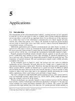
Figures 4-10 and 4-11 show the simulated SNR degradation in dB for different bit error
rates (BERs) versus the frequency error and timing error for QPSK, respectively. These
diagrams show that an OFDM system is sensitive to frequency and to clock errors. In order
to keep an acceptable performance degradation the error after frequency synchronization
and time synchronization should not exceed the following limits [68]:
τ
error
/T
s
< 0.01
f
error
T
s
< 0.02
(4.28)

Thus, the error relative to the sampling period should fulfill τ
error
/(N
c
T
samp
)<0.01 and
the error relative to the sub-carrier spacing shall not be greater than 2% of the sub-carrier
spacing, where the last is usually a quite difficult condition.
It should be noticed that for dimensioning the length of the guard time, the time
synchronization inaccuracy should be taken into account. As long as the sum of the
timing offset and the maximum multipath propagation delay is smaller than the guard
time, the only effect is a phase rotation that can be estimated by the channel estimator
(see Section 4.3) and compensated for by the channel equalizer (see Section 4.5).
4.2.3 Maximum Likelihood Parameter Estimation
Let us consider a frequency error f
error
and a timing error τ
error
. The joint maximum
likelihood estimates
ˆ
f
error
of the frequency error and ˆτ
error
of the timing error are obtained
by the maximization of the log-likelihood function (LLF ) as follows [10][55][73],
LLF(f
error

,τ
error
) = log p(r|f
error
,τ
error
), (4.29)
where p(r|f
error
,τ
error
) denotes the probability density function of observing the received
signal r, given a frequency error f
error
and timing error τ
error
. In [73] it is shown that for
130 Implementation Issues
0
0.5
1
1.5
2
2.5
3
3.5
0 0.02 0.04 0.06 0.08 0.1
SNR Degradation in dB
Frequency-error × T
s

BER = 10E − 04
BER = 10E − 02
Figure 4-10 SNR degradation in dB versus the normalized frequency error f
error
T
s
; N
c
= 2048
sub-carriers
0
2
4
6
8
10
12
0 0.005 0.01 0.015 0.02 0.025 0.03 0.035 0.04
SNR Degradation in dB
Clock-error/T
s
BER = 10E − 04
BER = 10E − 02
Figure 4-11 SNR degradation in dB versus the normalized timing error τ
error
/T
s
; N
c
= 2048

sub-carriers
Synchronization 131
N
c
+ M samples
LLF (f
error
,τ
error
) =|γ(τ
error
)| cos(2πf
error
+

γ(τ
error
)) − ρ(τ
error
) (4.30)
γ(m)=
m+M−1

k=m
r(k)r
∗
(k + N
c
), (m) =
m+M−1


k=m
|r(k)|
2
+|r(k+ N
c
)|
2
(4.31)
where

represents the argument of a complex number, ρ is a constant depending on the
SNR which represents the magnitude of the correlation between the sequences r(k) and
r(k+ N
c
),andm is the start of the correlation function of the received sequence (in case
of no timing error one can start at m = 0). Note that the first term in Eq. (4.30) is the
weighted-magnitude of γ(τ
error
), which is the sum of M consecutive correlations.
These sequences r(k) could be known in the receiver by transmitting, for instance, two
consecutive reference symbols (M = N
c
) as proposed by Moose [55] or one can exploit
the presence of the guard time (M = L
g
) [73].
The maximization of the above LLF can be done in two steps:
— a first maximization can be performed to find the frequency error estimate
ˆ

f
error
,
— then, the value of the given frequency error estimate is exploited for final maximization
to find the timing error estimate ˆτ
error
.
The maximization of f
error
is given by the partial derivation ∂LLF (f
error
,τ
error
)/∂f
error
=
0, which results in
ˆ
f
error
=−
1
2π

γ(τ
error
) + z =−
1
2π
m+M−1


k=m
Im[r(k)r
∗
(k + N
c
)]
m+M−1

k=m
Re[r(k)r
∗
(k + N
c
)]
+ z, (4.32)
where z is an integer value.
By inserting
ˆ
f
error
in Eq. (4.30), we obtain
LLF (
ˆ
f
error
,τ
error
) =|γ(τ
error

)|−ρ(τ
error
)(4.33)
and maximizing Eq. (4.33) gives us a joint estimate of
ˆ
f
error
and ˆτ
error
ˆ
f
error
=−
1
2π

γ(ˆτ
error
),
ˆτ
error
= arg(max
τ
error
{|γ(τ
error
)|−ρ(τ
error
)}. (4.34)
Note that in case of M = N

c
(i.e, two reference symbols), |
ˆ
f
error
| < 0.5, z = 0, and
no timing error τ
error
= 0(m = 0), one obtains the same results as Moose [55] (see
Figure 4-12).
The main drawback of the Moose maximum likelihood frequency detection is the small
range of acquisition which is only half of the sub-carrier spacing F
s
.Whenf
error
→
0.5F
s
, the estimate
ˆ
f
error
may, due to noise and the discontinuity of arctangent, jump
to −0.5. When this happens, the estimate is no longer unbiased and in practice it becomes
132 Implementation Issues
Delay N
c
arctang(.)
r(k)
estimated

frequency
error
1st OFDM Ref. Symbol
2nd OFDM Ref. Symbol
Time domain processing
FFT
( . )*
Figure 4-12 Moose maximum likelihood frequency estimator (M = N
c
)
useless. Thus, for frequency errors exceeding one half of the sub-carrier spacing, an
initial acquisition strategy, coarse frequency acquisition, should be applied. To enlarge
the acquisition range of a maximum likelihood estimator, a modified version of this
estimator was proposed in [10]. The basic idea is to modify the shape of the LLF.
The joint estimation of frequency and timing error using guard time may be sensitive in
environments with several long echoes. In the following section, we will examine some
approaches for time and frequency synchronization which are used in several implemen-
tations.
4.2.4 Time Synchronization
As we have explained before, the main objective of time synchronization for OFDM
systems is to know when a received OFDM symbol starts. By using the guard time the
timing requirements can be relaxed. A time offset, not exceeding the guard time, gives
rise to a phase rotation of the sub-carriers. This phase rotation is larger on the edge of the
frequency band. If a timing error is small enough to keep the channel impulse response
within the guard time, the orthogonality is maintained and a symbol timing delay can
be viewed as a phase shift introduced by the channel. This phase shift can be estimated
by the channel estimator (see Section 4.3) and corrected by the channel equalizer (see
Section 4.5). However, if a time shift is larger than the guard time, ISI and ICI occur and
signal orthogonality is lost.
Basically the task of the time synchronization is to estimate the two main functions: FFT

window positioning (OFDM symbol/frame synchronization) and sampling rate estimation
for A/D conversion controlling.
The operation of time synchronization can be carried out in two steps: Coarse and fine
symbol timing.
4.2.4.1 Coarse Symbol Timing
Different methods, depending on the transmission signal characteristics, can be used for
coarse timing estimation [22][23][73].
Basically, the power at baseband can be monitored prior to FFT processing and for
instance the dips resulting from null symbols (see Figure 4-9) might be used to control
Synchronization 133
a ‘flywheel’-type state transition algorithm as known from traditional frame synchroniza-
tion [40].
Null Symbol Detection
A null symbol, containing no power, is transmitted for instance in DAB at the beginning
of each OFDM frame (see Figure 4-13). By performing a simple power detection at the
receiver side before the FFT operation, the beginning of the frame can be detected. That
is, the receiver locates the null symbol by searching for a dip in the power of the received
signal. This can be achieved, for instance, by using a flywheel algorithm to guard against
occasional failures to detect the null symbol once in lock [40]. The basic function of
this algorithm is that, when the receiver is out of lock, it searches continuously for the
null symbols, whereas when in lock it searches for the symbol only at the expected null
symbols. The null symbol detection gives only a coarse timing information.
Two Identical Half Reference Symbols
In [76] a timing synchronization is proposed that searches for a training symbol with two
identical halves in the time domain, which can be sent at the beginning of an OFDM frame
(see Figure 4-14). At the receiver side, these two identical time domain sequences may
Tx OFDM frame
Null symbol = no Tx power
Received power
No power detected =

start of an OFDM frame
Power detected
Figure 4-13 Coarse time synchronization based on null symbol detection
r
(
k
)
estimated
timing offset
( . )*
1/2 OFDM ref. symb.
1/2 OFDM ref. symb.
|M(d)|
2
Power
estimation
metric |M
(
d)|
2
timing error
FFT
Time domain processing
Delay N
c
/2
Figure 4-14 Time synchronization based on two identical half reference symbols
134 Implementation Issues
only be phase shifted φ = πT
s

f
error
due to the carrier frequency offset. The two halves
of the training symbol are made identical by transmitting a PN sequence on the even
frequencies, while zeros are used on the odd frequencies. Let there be M complex-valued
samples in each half of the training symbol. The function for estimating the timing error
d is defined as
M(d)=
M−1

m=0
r
∗
d+m
r
d+m+M
M−1

m=0
|r
d+m+M
|
2
.(4.35)
Finally, the estimate of the timing error is derived by taking the maximum quadratic
value of the above function, i.e., max |M(d)|
2
. The main drawback of this metric is its
‘plateau’ which may lead to some uncertainties.
Guard Time Exploitation

Each OFDM symbol is extended by a cyclic repetition of the transmitted data (see
Figure 4-15). As the guard interval is just a duplication of a useful part of the OFDM
symbol, a correlation of the part containing the cyclic extension (guard interval) with the
given OFDM symbol enables a fast time synchronization [73]. The sampling rate can
also be estimated based on this correlation method. The presence of strong noise or long
echoes may prevent accurate symbol timing. However, the noise effect can be reduced
by integration (filtering) on several peaks obtained from subsequent estimates. As far as
echoes are concerned, if the guard time is chosen long enough to absorb all echoes, this
technique can still be reliable.
4.2.4.2 Fine Symbol Timing
For fine time synchronization, several methods based on transmitted reference symbols can
be used [12]. One straightforward solution applies the estimation of the channel impulse
response. The received signal without noise r(t)= s(t)⊗ h(t) is the convolution of the
transmit signal s(t) and the channel impulse response h(t). In the frequency domain after
FFT processing we obtain R(f ) = S(f )H(f). By transmitting special reference symbols
OFDM symbol
with guard time
Guard
time
Correlation with last
part of OFDM symbol
Cyclic extension
= same information
Cyclic extension
= same information
Correlation peak
= start of an OFDM
symbol
Figure 4-15 Time synchronization based on guard time correlation properties
Synchronization 135

(e.g., CAZAC sequences), S(f ) is apriori known by the receiver. Hence, after dividing
R(f ) by S(f ) and IFFT processing, the channel impulse response h(t) is obtained and
an accurate timing information can be derived.
If the FFT window is not properly positioned, the received signal becomes
r(t) = s(t − t
0
) ⊗ h(t), (4.36)
which turns into
R(f ) = S(f)H(f)e
−j 2πf t
0
(4.37)
after the FFT operation. After division of R(f ) by S(f) and again performing an IFFT, the
receiver obtains h(t − t
0
) and with that t
0
. Finally, the fine time synchronization process
consists of delaying the FFT window so that t
0
becomes quasi zero (see Figure 4-16).
In case of multipath propagation, the channel impulse response is made up of multiple
Dirac pulses. Let C
p
be the power of each constructive echo path and I
p
be the power of
a destructive path. An optimal time synchronization process is to maximize the C/I, the
ratio of the total constructive path power to the total destructive path power. However,
for ease of implementation a sub-optimal algorithm might be considered, where the FFT

window positioning signal uses the first significant echo, i.e., the first echo above a fixed
threshold. The threshold can be chosen from experience, but a reasonable starting value
can be derived from the minimum carrier-to-noise ratio required.
4.2.4.3 Sampling Clock Adjustment
As we have seen, the received analog signal is first sampled at instants determined by the
receiver clock before FFT operation. The effect of a clock frequency offset is twofold:
the useful signal component is rotated and attenuated and, furthermore, ICI is introduced.
The sampling clock could be considered to be close to its theoretical value so it may
have no effect on the result of the FFT. However, if the oscillator generating this clock
is left free-running, the window opened for FFT may gently slide and will not match the
useful interval of the symbols.
Guard
time
Symbol time
FFT window properly
positioned
FFT window with t
0
time difference
t
0
t
Time domain processing Frequency domain processing
Signal constellation
f = 0
f = 2pft
0
Figure 4-16 Fine time synchronization based on channel impulse response estimation
136 Implementation Issues
A first simple solution is to use the methods described above to evaluate the proper

position of the window and to dynamically readjust it. However, this method gener-
ates a phase discontinuity between symbols where a readjustment of the FFT win-
dow occurs. This phase discontinuity requires additional filtering or interpolation after
FFT operation.
A second method, although using a similar strategy, is to evaluate the shift of the FFT
window that is proportional to the frequency offset of the clock oscillator. The shift can be
used to control the oscillator with better accuracy. This method allows a fine adjustment
of the FFT window without the drawback of phase discontinuity from one symbol to
the other.
4.2.5 Frequency Synchronization
Another fundamental function of an OFDM receiver is the carrier frequency synchro-
nization. Frequency offsets are introduced by differences in oscillator frequencies in the
transmitter and receiver, Doppler shifts and phase noise. As we have seen earlier, the
frequency offset leads to a reduction of the signal amplitude since the sinc functions
are shifted and no longer sampled at the peak and to a loss of orthogonality between
sub-carriers. This loss introduces ICI which results in a degradation of the global system
performance [55][70][71].
In the previous sections we have seen that in order to avoid severe SNR degradation,
the frequency synchronization accuracy should be better than 2%. Note that a multi-carrier
system is much more sensitive to a frequency offset than a single carrier system [62].
As shown in Figure 4-8, the frequency error in an OFDM system is often corrected
by a tracking loop with a frequency detector to estimate the frequency offset. Depending
on the characteristics of the transmitted signal (pilot-based or not) several algorithms for
frequency detection and synchronization can be applied:
— algorithms based on the analysis of special synchronization symbols embedded in the
OFDM frame [7][50][55][58][76],
— algorithms based on the analysis of the received data at the output of the FFT (non-pilot
aided) [10], and
— algorithms based on the analysis of guard time redundancy [11][35][73].
Like the time synchronization, the frequency synchronization can be performed in two

steps: coarse and fine frequency synchronization.
4.2.5.1 Coarse Frequency Synchronization
We assume that the frequency offset is greater than half of the sub-carrier spacing, i.e.,
f
error
=
2z
T
s
+
φ
πT
s
,(4.38)
where the first term of the above equation represents the frequency offset which is a
multiple of the sub-carrier spacing where z is an integer and the second term is the
additional frequency offset being a fraction of the sub-carrier spacing, i.e., φ is smaller
than π .
Synchronization 137
The aim of the coarse frequency estimation is mainly to estimate z. Depending on the
transmitted OFDM signal, different approaches for coarse frequency synchronization can
be used [10][11][12][58][73][76].
CAZAC/M Sequences
A general approach is to analyze the transmitted special reference symbols at the begin-
ning of an OFDM frame; for instance, the CAZAC/M sequences [58] specified in the
DVB-T standard [16]. As shown in Figure 4-17, CAZAC/M sequences are generated in
the frequency domain and are embedded in I and R sequences. The CAZAC/M sequences
are differentially modulated. The length of the M sequences is much larger than the length
of the CAZAC sequences. The I and R sequences have the same length N
1

, where in the
I sequence (resp. R sequence) the imaginary (resp. real) components are 1 and the real
(resp. imaginary) components are 0. The I and R sequences are used as start positions for
the differential encoding/decoding of M sequences. A wide range coarse synchronization
is achieved by correlating with the transmitted known M sequence reference data, shifted
over ±N
1
sub-carriers (e.g., N
1
= 10 to 20) from the expected center point [22][58]. The
results from different sequences are averaged. The deviation of the correlation peak from
the expected center point z with −N
1
<z<+N
1
is converted to an equivalent value
used to correct the offset of the RF oscillator, or the baseband signal is corrected before
the FFT operation. This process can be repeated until the deviation is less than ±N
2
sub-
carriers (e.g., N
2
= 2 to 5). For a fine-range estimation, in a similar manner the remaining
CAZAC sequences can be applied that may reduce the frequency error to a few hertz.
The main advantage of this method is that it only uses one OFDM reference symbol.
However, its drawback is the high amount of computation needed, which may not be
adequate for burst transmission.
Schmidl and Cox
Similar to Moose [55], Schmidl and Cox [76] propose the use of two OFDM symbols for
frequency synchronization (see Figure 4-18). However, these two OFDM symbols have

a special construction which allows a frequency offset estimation greater than several
sub-carrier spacings. The first OFDM training symbol in the time domain consists of
two identical symbols generated in the frequency domain by a PN sequence on the even
r(k)
FFT
I, M, M, CAZAC, CAZAC, ..., CAZAC, M, M, R
Transmitted single OFDM reference symbol:
CAZAC/M
Extraction
and
diff. demod.
M-Seq. 1, z
M-Seq. 4, z
Averaging
and
searching
for max
z
frequency offset
z/T
s
Frequency domain processing
Figure 4-17 Coarse frequency offset estimation based on CAZAC/M sequences
138 Implementation Issues
FFT
Transmitted 2 ref. symbols in frequency
Ref. symb.
diff. demod.
of PN1
frequency

offset
2z/T
s
- PN1 in even sub-carriers
- PN2 in odd sub-carriers
2. Ref. symb.
Transmitted first ref. symb. in time
1/2 OFDM symb.
1/2 OFDM symb.
r(k)
Phase
correc.
[ . ]*
1/2 OFDM Ref. symb.
1/2 OFDM Ref. symb.
Delay
N
c
- PN1 in even sub-carriers
- zero in odd sub-carriers
1. Ref. symb.
1. Ref. symb.
2. Ref. symb. 1. Ref. symb.
B(z)
Phase
estim.
Frequency processing
Time processing
Power
estim.

Delay
N
c
/2
Power
estim.
Figure 4-18 Schmidl and Cox frequency offset estimation using 2 OFDM symbols
sub-carriers and zeros on the odd sub-carriers. The second training symbol contains a
differentially modulated PN sequence on the odd sub-carriers and another PN sequence
on the even sub-carriers. Note that the selection of a particular PN sequence has little
effect on the performance of the synchronization.
In Eq. (4.38), the second term can be estimated in a similar way to the Moose approach
[55] by employing the two halves of the first training symbols,
ˆ
φ = angle[M(d)](see
(4.35)). These two training symbols are frequency-corrected by
ˆ
φ/(πT
s
). Let their FFT
be x
1,k
and x
2,k
and let the differentially modulated PN sequence on the even frequencies
of the second training symbol be v
k
and let X be the set of indices for the even sub-
carriers. For the estimation of the integer sub-carrier offset given by z, the following
metric is calculated,

B(z) =





k∈X
x
∗
1,k+2z
v
∗
k
x
2,k+2z




2
2


k∈X
|x
2,k
|
2

2

.(4.39)
The estimate of z is obtained by taking the maximum value of the above metric B(z).
The main advantage of this method is its simplicity, which may be adequate for burst
transmission. Furthermore, it allows a joint estimation of timing and frequency offset (see
Section 4.2.4.1).
4.2.5.2 Fine Frequency Synchronization
Under the assumption that the frequency offset is less than half of the sub-carrier spacing,
there is a one-to-one correspondence between the phase rotation and the frequency offset.
The phase ambiguity limits the maximum frequency offset value. The phase offset can
be estimated by using pilot/reference aided algorithms [76].
Channel Estimation 139
FFT
Deframing
Coarse
carrier
frequency
estimation
Channel
estimation
Fine frequency
synchronization
Common
phase error
Pilots and references
r(k)
Figure 4-19 Frequency synchronization using reference symbols
Furthermore, as explained in Section 4.2.5.1, for fine frequency synchronization some
other reference data (i.e., CAZAC sequences) can be used. Here, the correlation process
in the frequency domain can be done over a limited number of sub-carrier frequencies
(e.g., ±N

2
sub-carriers).
As shown in Figure 4-19, channel estimation (see Section 4.3) can additionally deliver
a common phase error estimation (see Section 4.7.1.3) which can be exploited for fine
frequency synchronization.
4.2.6 Automatic Gain Control (AGC)
In order to maximize the input signal dynamic by avoiding saturation, the variation of
the received signal field strength before FFT operation or before A/D conversion can be
adjusted by an AGC function [12][76]. Two kinds of AGC can be implemented:
— Controlling the time domain signal before A/D conversion: First, in the digital domain,
the average received power is computed by filtering. Then, the output signal is con-
verted to analog (e.g., by a sigma-delta modulator) that controls the signal attenuation
before the A/D conversion.
— Controlling the time domain signal before FFT: In the frequency domain the output of
the FFT signal is analyzed and the result is used to control the signal before the FFT.
4.3 Channel Estimation
When applying receivers with coherent detection in fading channels, information about
the channel state is required and has to be estimated by the receiver. The basic princi-
ple of pilot symbol aided channel estimation is to multiplex reference symbols, so-called
pilot symbols, into the data stream. The receiver estimates the channel state informa-
tion based on the received, known pilot symbols. The pilot symbols can be scattered
in time and/or frequency direction in OFDM frames (see Figure 4-9). Special cases are
either pilot tones which are sequences of pilot symbols in time direction on certain sub-
carriers, or OFDM reference symbols which are OFDM symbols consisting completely
of pilot symbols.