General Random Variables
Bạn đang xem bản rút gọn của tài liệu. Xem và tải ngay bản đầy đủ của tài liệu tại đây (195.52 KB, 8 trang )
Chapter 11
General Random Variables
11.1 Law of a Random Variable
Thus far we have considered only random variables whose domain and range are discrete. We now
consider a general random variable
X :!IR
defined on the probability space
; F ; P
. Recall
that:
F
is a
-algebra of subsets of
.
IP is a probability measure on
F
, i.e.,
IP A
is defined for every
A 2F
.
A function
X :!IR
is a random variable if and only if for every
B 2BIR
(the
-algebra of
Borel subsets of IR), the set
fX 2 B g
4
= X
,1
B
4
= f! ; X ! 2 B g2F;
i.e.,
X :!IR
is a random variable if and only if
X
,1
is a function from
BIR
to
F
(See Fig.
11.1)
Thus any random variable
X
induces a measure
X
on the measurable space
IR; BIR
defined
by
X
B =IP
X
,1
B
8B 2BIR;
where the probabiliy on the right is defined since
X
,1
B 2F
.
X
is often called the Law of
X
–
in Williams’ book this is denoted by
L
X
.
11.2 Density of a Random Variable
The density of
X
(if it exists) is a function
f
X
: IR!0; 1
such that
X
B =
Z
B
f
X
xdx 8B 2BIR:
123
124
R
Ω
B}ε
B
X
{X
Figure 11.1: Illustrating a real-valued random variable
X
.
We then write
d
X
x=f
X
xdx;
where the integral is with respect to the Lebesgue measure on IR.
f
X
is the Radon-Nikodym deriva-
tive of
X
with respect to the Lebesgue measure. Thus
X
has a density if and only if
X
is
absolutely continuous with respect to Lebesgue measure, which means that whenever
B 2BIR
has Lebesgue measure zero, then
IP fX 2 B g =0:
11.3 Expectation
Theorem 3.32 (Expectation of a function of
X
) Let
h : IR!IR
be given. Then
IEhX
4
=
Z
hX! dIP !
=
Z
IR
hx d
X
x
=
Z
IR
hxf
X
x dx:
Proof: (Sketch). If
hx=1
B
x
for some
B IR
, then these equations are
IE 1
B
X
4
= P fX 2 B g
=
X
B
=
Z
B
f
X
x dx;
which are true by definition. Now use the “standard machine” to get the equations for general
h
.
CHAPTER 11. General Random Variables
125
Ω
ε
(X,Y)
{ (X,Y) C}
C
x
y
Figure 11.2: Two real-valued random variables
X; Y
.
11.4 Two random variables
Let
X; Y
be two random variables
!IR
defined on the space
; F ; P
.Then
X; Y
induce a
measure on
BIR
2
(see Fig. 11.2) called the joint law of
X; Y
,definedby
X;Y
C
4
= IP fX; Y 2 C g 8C 2BIR
2
:
The joint density of
X; Y
is a function
f
X;Y
: IR
2
!0; 1
that satisfies
X;Y
C=
ZZ
C
f
X;Y
x; y dxdy 8C 2BIR
2
:
f
X;Y
is the Radon-Nikodym derivative of
X;Y
with respect to the Lebesgue measure (area) on
IR
2
.
We compute the expectation of a function of
X; Y
in a manner analogous to the univariate case:
IEkX; Y
4
=
Z
kX !;Y! dIP !
=
ZZ
IR
2
kx; y d
X;Y
x; y
=
ZZ
IR
2
kx; y f
X;Y
x; y dxdy
126
11.5 Marginal Density
Suppose
X; Y
has joint density
f
X;Y
.Let
B IR
be given. Then
Y
B = IP fY 2 B g
= IP fX; Y 2 IR Bg
=
X;Y
IR B
=
Z
B
Z
IR
f
X;Y
x; y dxdy
=
Z
B
f
Y
y dy ;
where
f
Y
y
4
=
Z
IR
f
X;Y
x; y dx:
Therefore,
f
Y
y
is the (marginal) density for
Y
.
11.6 Conditional Expectation
Suppose
X; Y
has joint density
f
X;Y
.Let
h : IR!IR
be given. Recall that
IE hX jY
4
=
IE hX jY
depends on
!
through
Y
, i.e., there is a function
g y
(
g
depending on
h
) such that
IE hX jY != gY!:
How do we determine
g
?
We can characterize
g
using partial averaging: Recall that
A 2 Y A = fY 2 B g
for some
B 2BIR
. Then the following are equivalent characterizations of
g
:
Z
A
g Y dIP =
Z
A
hX dIP 8A 2 Y ;
(6.1)
Z
1
B
Y g Y dIP =
Z
1
B
Y hX dIP 8B 2BIR;
(6.2)
Z
IR
1
B
y g y
Y
dy =
ZZ
IR
2
1
B
yhx d
X;Y
x; y 8B 2BIR;
(6.3)
Z
B
g y f
Y
y dy =
Z
B
Z
IR
hxf
X;Y
x; y dxdy 8B 2BIR:
(6.4)
CHAPTER 11. General Random Variables
127
11.7 Conditional Density
A function
f
X jY
xjy :IR
2
!0; 1
is called a conditional density for
X
given
Y
provided that for
any function
h : IR!IR
:
g y =
Z
IR
hxf
XjY
xjydx:
(7.1)
(Here
g
is the function satisfying
IE hX jY =gY;
and
g
depends on
h
,but
f
X jY
does not.)
Theorem 7.33 If
X; Y
has a joint density
f
X;Y
,then
f
X jY
xjy=
f
X;Y
x; y
f
Y
y
:
(7.2)
Proof: Just verify that
g
defined by (7.1) satisfies (6.4): For
B 2BIR;
Z
B
Z
IR
hxf
XjY
xjydx
| z
gy
f
Y
y dy =
Z
B
Z
IR
hxf
X;Y
x; y dxdy :
Notation 11.1 Let
g
be the function satisfying
IE hX jY =gY:
The function
g
is often written as
g y = IEhXjY = y;
and (7.1) becomes
IE hX jY = y =
Z
IR
hxf
XjY
xjydx:
In conclusion, to determine
IE hX jY
(a function of
!
), first compute
g y =
Z
IR
hxf
XjY
xjydx;
and then replace the dummy variable
y
by the random variable
Y
:
IE hX jY != gY!:
Example 11.1 (Jointly normal random variables) Given parameters:
1
0;
2
0;,1 1
.Let
X; Y
have the joint density
f
X;Y
x; y=
1
2
1
2
p
1 ,
2
exp
,
1
21 ,
2
x
2
2
1
, 2
x
1
y
2
+
y
2
2
2
: