Stopping Times and American Options
Bạn đang xem bản rút gọn của tài liệu. Xem và tải ngay bản đầy đủ của tài liệu tại đây (168.7 KB, 8 trang )
Chapter 5
Stopping Times and American Options
5.1 American Pricing
Let us first review the European pricing formula in a Markov model. Consider the Binomial
model with
n
periods. Let
V
n
= g S
n
be the payoff of a derivative security. Define by backward
recursion:
v
n
x = g x
v
k
x =
1
1+r
~pv
k+1
ux+ ~qv
k+1
dx:
Then
v
k
S
k
is the value of the option at time
k
, and the hedging portfolio is given by
k
=
v
k+1
uS
k
, v
k+1
dS
k
u , dS
k
; k =0;1;2;::: ;n , 1:
Now consider an American option. Again a function
g
is specified. In any period
k
, the holder
of the derivative security can “exercise” and receive payment
g S
k
. Thus, the hedging portfolio
should create a wealth process which satisfies
X
k
g S
k
; 8k;
almost surely.
This is because the value of the derivative security at time
k
is at least
g S
k
, and the wealth process
value at that time must equal the value of the derivative security.
American algorithm.
v
n
x = g x
v
k
x = max
1
1+r
~pv
k+1
ux+ ~qv
k+1
dx;gx
Then
v
k
S
k
is the value of the option at time
k
.
77
78
v (16) = 0
2
S = 4
0
S (H) = 8
S (T) = 2
S (HH) = 16
S (TT) = 1
S (HT) = 4
S (TH) = 4
1
1
2
2
2
2
v (4) = 1
v (1) = 4
2
2
Figure 5.1: Stock price and final value of an American put option with strike price 5.
Example 5.1 See Fig. 5.1.
S
0
=4;u =2;d =
1
2
;r =
1
4
; ~p =~q=
1
2
;n =2
.Set
v
2
x=gx=5,x
+
.
Then
v
1
8 = max
4
5
1
2
:0+
1
2
:1
;5 , 8
+
= max
2
5
; 0
= 0:40
v
1
2 = max
4
5
1
2
:1+
1
2
:4
;5 , 2
+
= maxf2; 3g
= 3:00
v
0
4 = max
4
5
1
2
:0:4 +
1
2
:3:0
; 5 , 4
+
= maxf1:36; 1g
= 1:36
Let us now construct the hedging portfolio for this option. Begin with initial wealth
X
0
=1:36
. Compute
0
as follows:
0:40 = v
1
S
1
H
= S
1
H
0
+1+rX
0
,
0
S
0
= 8
0
+
5
4
1:36 , 4
0
= 3
0
+1:70 =
0
= ,0:43
3:00 = v
1
S
1
T
= S
1
T
0
+1+rX
0
,
0
S
0
= 2
0
+
5
4
1:36 , 4
0
= ,3
0
+1:70 =
0
= ,0:43
CHAPTER 5. Stopping Times and American Options
79
Using
0
= ,0:43
results in
X
1
H =v
1
S
1
H = 0:40;X
1
T=v
1
S
1
T=3:00
Now let us compute
1
(Recall that
S
1
T =2
):
1 = v
2
4
= S
2
TH
1
T + 1 + rX
1
T ,
1
T S
1
T
= 4
1
T +
5
4
3 , 2
1
T
= 1:5
1
T +3:75 =
1
T =,1:83
4 = v
2
1
= S
2
TT
1
T + 1 + rX
1
T ,
1
T S
1
T
=
1
T +
5
4
3 , 2
1
T
= ,1:5
1
T +3:75 =
1
T =,0:16
We get different answers for
1
T
!Ifwehad
X
1
T =2
, the value of the European put, we would have
1=1:5
1
T +2:5=
1
T=,1;
4=,1:5
1
T +2:5=
1
T=,1;
5.2 Value of Portfolio Hedging an American Option
X
k+1
=
k
S
k+1
+1+rX
k
, C
k
,
k
S
k
= 1 + rX
k
+
k
S
k+1
, 1 + rS
k
, 1 + rC
k
Here,
C
k
is the amount “consumed” at time
k
.
The discounted value of the portfolio is a supermartingale.
The value satisfies
X
k
g S
k
;k =0;1;::: ;n
.
The value process is the smallest process with these properties.
When do you consume? If
f
IE 1 + r
,k+1
v
k+1
S
k+1
jF
k
1 + r
,k
v
k
S
k
;
or, equivalently,
f
IE
1
1+r
v
k+1
S
k+1
jF
k
v
k
S
k
80
and the holder of the American option does not exercise, then the seller of the option can consume
to close the gap. By doing this, he can ensure that
X
k
= v
k
S
k
for all
k
,where
v
k
is the value
defined by the American algorithm in Section 5.1.
In the previous example,
v
1
S
1
T =3;v
2
S
2
TH = 1
and
v
2
S
2
TT = 4
. Therefore,
f
IE
1
1+ r
v
2
S
2
jF
1
T =
4
5
h
1
2
:1+
1
2
:4
i
=
4
5
5
2
= 2;
v
1
S
1
T = 3;
so there is a gap of size 1. If the owner of the option does not exercise it at time one in the state
!
1
= T
, then the seller can consume 1 at time 1. Thereafter, he uses the usual hedging portfolio
k
=
v
k+1
uS
k
, v
k+1
dS
k
u , dS
k
In the example, we have
v
1
S
1
T = g S
1
T
. It is optimal for the owner of the American option
to exercise whenever its value
v
k
S
k
agrees with its intrinsic value
g S
k
.
Definition 5.1 (Stopping Time) Let
; F ; P
be a probability space and let
fF
k
g
n
k=0
be a filtra-
tion. A stopping time is a random variable
:!f0; 1; 2;::: ;ng f1g
with the property that:
f! 2 ; != kg2F
k
; 8k=0;1;::: ;n;1:
Example 5.2 Consider the binomial model with
n =2;S
0
=4;u =2;d =
1
2
;r =
1
4
,so
~p =~q=
1
2
.Let
v
0
;v
1
;v
2
be the value functions defined for the American put with strike price 5. Define
! = minfk; v
k
S
k
=5,S
k
+
g:
The stopping time
corresponds to “stopping the first time the value of the option agrees with its intrinsic
value”. It is an optimal exercise time. We note that
!=
1
if
! 2 A
T
2
if
! 2 A
H
We verify that
is indeed a stopping time:
f! ; !=0g = 2F
0
f!;!=1g = A
T
2F
1
f!;!=2g = A
H
2F
2
Example 5.3 (A random time which is not a stopping time) In the same binomialmodel as in the previous
example, define
! = minfk; S
k
!=m
2
!g;
CHAPTER 5. Stopping Times and American Options
81
where
m
2
4
= min
0j 2
S
j
.Inotherwords,
stops when the stock price reaches its minimum value. This
random variable is given by
! =
8
:
0
if
! 2 A
H
;
1
if
! = TH;
2
if
! = TT
We verify that
is not a stopping time:
f!; !=0g = A
H
62 F
0
f!; !=1g = fTHg62 F
1
f!;!=2g = fTTg2F
2
5.3 Information up to a Stopping Time
Definition 5.2 Let
be a stopping time. We say that a set
A
is determined by time
provided
that
A f!;!=kg2F
k
;8k:
The collection of sets determined by
is a
-algebra, which we denote by
F
.
Example 5.4 In the binomial model considered earlier, let
= minfk; v
k
S
k
=5,S
k
+
g;
i.e.,
!=
1
if
! 2 A
T
2
if
! 2 A
H
The set
fHT g
is determined by time
,buttheset
fTHg
is not. Indeed,
fHT gf!;!=0g = 2F
0
fHT gf!;!=1g = 2F
1
fHT gf!;!=2g = fHT g2F
2
but
fTHgf!;!=1g=fTHg62F
1
:
The atoms of
F
are
fHT g; fHHg;A
T
=fTH;TTg:
Notation 5.1 (Value of Stochastic Process at a Stopping Time) If
; F ; P
is a probabilityspace,
fF
k
g
n
k=0
is a filtration under
F
,
fX
k
g
n
k=0
is a stochastic process adapted to this filtration, and
is
a stopping time with respect to the same filtration, then
X
is an
F
-measurable random variable
whose value at
!
is given by
X
!
4
= X
!
! :