The Markov Property
Bạn đang xem bản rút gọn của tài liệu. Xem và tải ngay bản đầy đủ của tài liệu tại đây (193.28 KB, 10 trang )
Chapter 4
The Markov Property
4.1 Binomial Model Pricing and Hedging
Recall that
V
m
is the given simple European derivative security, and the value and portfolio pro-
cesses are given by:
V
k
=1+r
k
f
IE1 + r
,m
V
m
jF
k
; k =0;1;::: ;m, 1:
k
!
1
;::: ;!
k
=
V
k+1
!
1
;::: ;!
k
;H, V
k+1
!
1
;::: ;!
k
;T
S
k+1
!
1
;::: ;!
k
;H, S
k+1
!
1
;::: ;!
k
;T
; k =0;1;::: ;m, 1:
Example 4.1 (Lookback Option)
u =2;d =0:5;r =0:25;S
0
=4;~p=
1+r,d
u,d
=0:5;~q=1,~p=0:5:
Consider a simple European derivative security with expiration 2, with payoff given by (See Fig. 4.1):
V
2
= max
0k2
S
k
, 5
+
:
Notice that
V
2
HH=11;V
2
HT =36=V
2
TH=0;V
2
TT=0:
The payoff is thus “path dependent”. Working backward in time, we have:
V
1
H =
1
1+r
~pV
2
HH+ ~qV
2
HT =
4
5
0:5 11 + 0:5 3 = 5:60;
V
1
T =
4
5
0:5 0+0:50 = 0;
V
0
=
4
5
0:5 5:60 + 0:5 0=2:24:
Using these values, we can now compute:
0
=
V
1
H , V
1
T
S
1
H , S
1
T
=0:93;
1
H =
V
2
HH , V
2
HT
S
2
HH , S
2
HT
=0:67;
67
68
S = 4
0
S (H) = 8
S (T) = 2
S (HH) = 16
S (TT) = 1
S (HT) = 4
S (TH) = 4
1
1
2
2
2
2
Figure 4.1: Stock price underlying the lookback option.
1
T =
V
2
TH , V
2
TT
S
2
TH , S
2
TT
=0:
Working forward in time, we can check that
X
1
H =
0
S
1
H + 1 + rX
0
,
0
S
0
=5:59; V
1
H =5:60;
X
1
T =
0
S
1
T + 1 + rX
0
,
0
S
0
=0:01; V
1
T =0;
X
1
HH=
1
HS
1
HH + 1 + rX
1
H ,
1
H S
1
H =11:01; V
1
HH=11;
etc.
Example 4.2 (European Call) Let
u =2;d =
1
2
;r =
1
4
;S
0
=4;~p=~q=
1
2
, and consider a European call
with expiration time 2 and payoff function
V
2
=S
2
,5
+
:
Note that
V
2
HH=11;V
2
HT =V
2
TH=0;V
2
TT=0;
V
1
H=
4
5
1
2
:11 +
1
2
:0=4:40
V
1
T =
4
5
1
2
:0+
1
2
:0 = 0
V
0
=
4
5
1
2
4:40 +
1
2
0 = 1:76:
Define
v
k
x
to be the value of the call at time
k
when
S
k
= x
.Then
v
2
x=x,5
+
v
1
x=
4
5
1
2
v
2
2x+
1
2
v
2
x=2;
v
0
x=
4
5
1
2
v
1
2x+
1
2
v
1
x=2:
CHAPTER 4. The Markov Property
69
In particular,
v
2
16 = 11;v
2
4 = 0;v
2
1 = 0;
v
1
8 =
4
5
1
2
:11 +
1
2
:0 = 4:40;
v
1
2 =
4
5
1
2
:0+
1
2
:0 = 0;
v
0
=
4
5
1
2
4:40 +
1
2
0 = 1:76:
Let
k
x
be the number of shares in the hedging portfolio at time
k
when
S
k
= x
.Then
k
x=
v
k+1
2x , v
k+1
x=2
2x , x=2
;k=0;1:
4.2 Computational Issues
For a model with
n
periods (coin tosses),
has
2
n
elements. For period
k
, we must solve
2
k
equations of the form
V
k
!
1
;::: ;!
k
=
1
1+r
~pV
k+1
!
1
;::: ;!
k
;H+ ~qV
k+1
!
1
;::: ;!
k
;T:
For example, a three-month option has 66 trading days. If each day is taken to be one period, then
n =66
and
2
66
7 10
19
.
There are three possible ways to deal with this problem:
1. Simulation. We have, for example, that
V
0
=1+r
,n
f
IEV
n
;
and so we could compute
V
0
by simulation. More specifically, we could simulate
n
coin
tosses
! =!
1
;::: ;!
n
under the risk-neutral probability measure. We could store the
value of
V
n
!
. We could repeat this several times and take the average value of
V
n
as an
approximation to
f
IEV
n
.
2. Approximate a many-period model by a continuous-time model. Then we can use calculus
and partial differential equations. We’ll get to that.
3. Look for Markov structure. Example 4.2 has this. In period 2, the option in Example 4.2 has
threepossiblevalues
v
2
16;v
2
4;v
2
1
, ratherthan four possiblevalues
V
2
HH;V
2
HT ;V
2
TH;V
2
TT
.
If there were 66 periods, then in period 66 there would be 67 possible stock price values(since
the final price depends only on the number of up-ticks of the stock price – i.e., heads – so far)
and hence only 67 possible option values, rather than
2
66
7 10
19
.
70
4.3 Markov Processes
Technical condition always present: We consider only functions on IR and subsets of IR which are
Borel-measurable, i.e., we only consider subsets
A
of IRthatarein
B
and functions
g : IR!IR
such
that
g
,1
is a function
B!B
.
Definition 4.1 () Let
; F ; P
be a probability space. Let
fF
k
g
n
k=0
be a filtration under
F
.Let
fX
k
g
n
k=0
be a stochastic process on
; F ; P
. This process is said to be Markov if:
The stochastic process
fX
k
g
is adapted to the filtration
fF
k
g
,and
(The Markov Property). For each
k =0;1;::: ;n , 1
, the distribution of
X
k+1
conditioned
on
F
k
is the same as the distribution of
X
k+1
conditioned on
X
k
.
4.3.1 Different ways to write the Markov property
(a) (Agreement of distributions). For every
A 2B
4
=BIR
,wehave
IP X
k+1
2 AjF
k
= IE I
A
X
k+1
jF
k
= IE I
A
X
k+1
jX
k
= IP X
k+1
2 AjX
k
:
(b) (Agreement of expectations of all functions). For every (Borel-measurable) function
h : IR!IR
for which
IE jhX
k+1
j 1
,wehave
IE hX
k+1
jF
k
=IEhX
k+1
jX
k
:
(c) (Agreement of Laplace transforms.) For every
u 2 IR
for which
IEe
uX
k+1
1
,wehave
IE
e
uX
k+1
F
k
= IE
e
uX
k+1
X
k
:
(If we fix
u
and define
hx=e
ux
, then the equations in (b) and (c) are the same. However in
(b) we have a condition which holds for every function
h
, and in (c) we assume this condition
onlyfor functions
h
of the form
hx=e
ux
. A main resultin the theory of Laplace transforms
is that if the equation holds for every
h
of this special form, then it holds for every
h
, i.e., (c)
implies (b).)
(d) (Agreement of characteristic functions) For every
u 2 IR
,wehave
IE
h
e
iuX
k+1
jF
k
i
= IE
h
e
iuX
k+1
jX
k
i
;
where
i =
p
,1
.(Since
je
iux
j = j cos x + sin xj1
we don’t need to assume that
IE je
iux
j
1
.)
CHAPTER 4. The Markov Property
71
Remark 4.1 In every case of the Markov properties where
IE :::jX
k
appears, we could just as
well write
g X
k
for some function
g
. For example, form (a) of the Markov property can be restated
as:
For every
A 2B
,wehave
IP X
k+1
2 AjF
k
=gX
k
;
where
g
is a function that depends on the set
A
.
Conditions (a)-(d) are equivalent. The Markov property as stated in (a)-(d) involves the process at
a “current” time
k
and one future time
k +1
. Conditions (a)-(d) are also equivalent to conditions
involving the process at time
k
and multiple future times. We write these apparently stronger but
actually equivalent conditions below.
Consequences of the Markov property. Let
j
be a positive integer.
(A) For every
A
k+1
IR;::: ;A
k+j
IR
,
IPX
k+1
2 A
k+1
;::: ;X
k+j
2 A
k+j
jF
k
=IPX
k+1
2 A
k+1
;::: ;X
k+j
2 A
k+j
jX
k
:
(A’) For every
A 2 IR
j
,
IP X
k+1
;::: ;X
k+j
2 AjF
k
=IPX
k+1
;::: ;X
k+j
2 AjX
k
:
(B) For every function
h : IR
j
!IR
for which
IE jhX
k+1
;::: ;X
k+j
j 1
,wehave
IE hX
k+1
;::: ;X
k+j
jF
k
=IEhX
k+1
;::: ;X
k+j
jX
k
:
(C) For every
u =u
k+1
;::: ;u
k+j
2 IR
j
for which
IE je
u
k+1
X
k+1
+:::+u
k+j
X
k+j
j 1
,wehave
IE e
u
k+1
X
k+1
+:::+u
k+j
X
k+j
jF
k
=IEe
u
k+1
X
k+1
+:::+u
k+j
X
k+j
jX
k
:
(D) For every
u =u
k+1
;::: ;u
k+j
2 IR
j
we have
IE e
iu
k+1
X
k+1
+:::+u
k+j
X
k+j
jF
k
=IEe
iu
k+1
X
k+1
+:::+u
k+j
X
k+j
jX
k
:
Once again, every expression of the form
IE :::jX
k
can also be written as
g X
k
,wherethe
function
g
depends on the random variable represented by
:::
in this expression.
Remark. All these Markov properties have analogues for vector-valued processes.