The variational bayes method in signal processing 2006
Bạn đang xem bản rút gọn của tài liệu. Xem và tải ngay bản đầy đủ của tài liệu tại đây (6.89 MB, 241 trang )
Springer Series on
Signals and Communication Technology
Signals and Communication Technology
Circuits and Systems
Based on Delta Modulation
Linear, Nonlinear and Mixed Mode Processing
D.G. Zrilic ISBN 3-540-23751-8
Functional Structures in Networks
AMLn – A Language for Model Driven
Development of Telecom Systems
T. Muth ISBN 3-540-22545-5
RadioWave Propagation
for Telecommunication Applications
H. Sizun ISBN 3-540-40758-8
Electronic Noise and Interfering Signals
Principles and Applications
G. Vasilescu ISBN 3-540-40741-3
DVB
The Family of International Standards
for Digital Video Broadcasting, 2nd ed.
U. Reimers ISBN 3-540-43545-X
Digital Interactive TV and Metadata
Future Broadcast Multimedia
A. Lugmayr, S. Niiranen, and S. Kalli
ISBN 3-387-20843-7
Adaptive Antenna Arrays
Trends and Applications
S. Chandran (Ed.) ISBN 3-540-20199-8
Digital Signal Processing
with Field Programmable Gate Arrays
U. Meyer-Baese ISBN 3-540-21119-5
Neuro-Fuzzy and Fuzzy Neural Applications
in Telecommunications
P. Stavroulakis (Ed.) ISBN 3-540-40759-6
SDMA for Multipath Wireless Channels
Limiting Characteristics
and Stochastic Models
I.P. Kovalyov ISBN 3-540-40225-X
Digital Television
A Practical Guide for Engineers
W. Fischer ISBN 3-540-01155-2
Multimedia Communication Technology
Representation, Transmission
and Identification of Multimedia Signals
J.R. Ohm ISBN 3-540-01249-4
Information Measures
Information and its Description in Science
and Engineering
C. Arndt ISBN 3-540-40855-X
Processing of SAR Data
Fundamentals, Signal Processing,
Interferometry
A. Hein ISBN 3-540-05043-4
Chaos-Based Digital
Communication Systems
Operating Principles, Analysis Methods,
and Performance Evalutation
F.C.M. Lau and C.K. Tse ISBN 3-540-00602-8
Adaptive Signal Processing
Application to Real-World Problems
J. Benesty and Y. Huang (Eds.)
ISBN 3-540-00051-8
Multimedia Information Retrieval
and Management
Technological Fundamentals and Applications
D. Feng, W.C. Siu, and H.J. Zhang (Eds.)
ISBN 3-540-00244-8
Structured Cable Systems
A.B. Semenov, S.K. Strizhakov,
and I.R. Suncheley ISBN 3-540-43000-8
UMTS
The Physical Layer of the Universal Mobile
Telecommunications System
A. Springer and R. Weigel
ISBN 3-540-42162-9
Advanced Theory of Signal Detection
Weak Signal Detection in
Generalized Obeservations
I. Song, J. Bae, and S.Y. Kim
ISBN 3-540-43064-4
Wireless Internet Access over GSM and UMTS
M. Taferner and E. Bonek
ISBN 3-540-42551-9
The Variational Bayes Method
in Signal Processing
ˇ ıdl and A. Quinn
V. Sm´
ISBN 3-540-28819-8
ˇ ıdl
V´aclav Sm´
Anthony Quinn
The Variational
Bayes Method
in Signal Processing
With 65 Figures
123
ˇ ıdl
Dr. V´aclav Sm´
Institute of Information Theory and Automation
Academy of Sciences of the Czech Republic, Department of Adaptive Systems
PO Box 18, 18208 Praha 8, Czech Republic
E-mail:
Dr. Anthony Quinn
Department of Electronic and Electrical Engineering
University of Dublin, Trinity College
Dublin 2, Ireland
E-mail:
ISBN-10 3-540-28819-8 Springer Berlin Heidelberg New York
ISBN-13 978-3-540-28819-0 Springer Berlin Heidelberg New York
Library of Congress Control Number: 2005934475
This work is subject to copyright. All rights are reserved, whether the whole or part of the material is
concerned, specif ically the rights of translation, reprinting, reuse of illustrations, recitation, broadcasting,
reproduction on microf ilm or in any other way, and storage in data banks. Duplication of this publication or
parts thereof is permitted only under the provisions of the German Copyright Law of September 9, 1965, in its
current version, and permission for use must always be obtained from Springer-Verlag. Violations are liable
to prosecution under the German Copyright Law.
Springer is a part of Springer Science+Business Media.
springer.com
© Springer-Verlag Berlin Heidelberg 2006
Printed in Germany
The use of general descriptive names, registered names, trademarks, etc. in this publication does not imply,
even in the absence of a specif ic statement, that such names are exempt from the relevant protective laws and
regulations and therefore free for general use.
Typesetting and production: SPI Publisher Services
Cover design: design & production GmbH, Heidelberg
Printed on acid-free paper
SPIN: 11370918
62/3100/SPI - 5 4 3 2 1 0
Do mo Thuismitheoirí
A.Q.
Preface
Gaussian linear modelling cannot address current signal processing demands. In
modern contexts, such as Independent Component Analysis (ICA), progress has been
made specifically by imposing non-Gaussian and/or non-linear assumptions. Hence,
standard Wiener and Kalman theories no longer enjoy their traditional hegemony in
the field, revealing the standard computational engines for these problems. In their
place, diverse principles have been explored, leading to a consequent diversity in the
implied computational algorithms. The traditional on-line and data-intensive preoccupations of signal processing continue to demand that these algorithms be tractable.
Increasingly, full probability modelling (the so-called Bayesian approach)—or
partial probability modelling using the likelihood function—is the pathway for design of these algorithms. However, the results are often intractable, and so the area
of distributional approximation is of increasing relevance in signal processing. The
Expectation-Maximization (EM) algorithm and Laplace approximation, for example, are standard approaches to handling difficult models, but these approximations
(certainty equivalence, and Gaussian, respectively) are often too drastic to handle
the high-dimensional, multi-modal and/or strongly correlated problems that are encountered. Since the 1990s, stochastic simulation methods have come to dominate
Bayesian signal processing. Markov Chain Monte Carlo (MCMC) sampling, and related methods, are appreciated for their ability to simulate possibly high-dimensional
distributions to arbitrary levels of accuracy. More recently, the particle filtering approach has addressed on-line stochastic simulation. Nevertheless, the wider acceptability of these methods—and, to some extent, Bayesian signal processing itself—
has been undermined by the large computational demands they typically make.
The Variational Bayes (VB) method of distributional approximation originates—
as does the MCMC method—in statistical physics, in the area known as Mean Field
Theory. Its method of approximation is easy to understand: conditional independence is enforced as a functional constraint in the approximating distribution, and
the best such approximation is found by minimization of a Kullback-Leibler divergence (KLD). The exact—but intractable—multivariate distribution is therefore factorized into a product of tractable marginal distributions, the so-called VB-marginals.
This straightforward proposal for approximating a distribution enjoys certain opti-
VIII
Preface
mality properties. What is of more pragmatic concern to the signal processing community, however, is that the VB-approximation conveniently addresses the following
key tasks:
1. The inference is focused (or, more formally, marginalized) onto selected subsets
of parameters of interest in the model: this one-shot (i.e. off-line) use of the VB
method can replace numerically intensive marginalization strategies based, for
example, on stochastic sampling.
2. Parameter inferences can be arranged to have an invariant functional form
when updated in the light of incoming data: this leads to feasible on-line
tracking algorithms involving the update of fixed- and finite-dimensional statistics. In the language of the Bayesian, conjugacy can be achieved under the
VB-approximation. There is no reliance on propagating certainty equivalents,
stochastically-generated particles, etc.
Unusually for a modern Bayesian approach, then, no stochastic sampling is required
for the VB method. In its place, the shaping parameters of the VB-marginals are
found by iterating a set of implicit equations to convergence. This Iterative Variational Bayes (IVB) algorithm enjoys a decisive advantage over the EM algorithm
whose computational flow is similar: by design, the VB method yields distributions
in place of the point estimates emerging from the EM algorithm. Hence, in common
with all Bayesian approaches, the VB method provides, for example, measures of
uncertainty for any point estimates of interest, inferences of model order/rank, etc.
The machine learning community has led the way in exploiting the VB method
in model-based inference, notably in inference for graphical models. It is timely,
however, to examine the VB method in the context of signal processing where, to
date, little work has been reported. In this book, at all times, we are concerned with
the way in which the VB method can lead to the design of tractable computational
schemes for tasks such as (i) dimensionality reduction, (ii) factor analysis for medical
imagery, (iii) on-line filtering of outliers and other non-Gaussian noise processes, (iv)
tracking of non-stationary processes, etc. Our aim in presenting these VB algorithms
is not just to reveal new flows-of-control for these problems, but—perhaps more
significantly—to understand the strengths and weaknesses of the VB-approximation
in model-based signal processing. In this way, we hope to dismantle the current psychology of dependence in the Bayesian signal processing community on stochastic
sampling methods. Without doubt, the ability to model complex problems to arbitrary
levels of accuracy will ensure that stochastic sampling methods—such as MCMC—
will remain the golden standard for distributional approximation. Notwithstanding
this, our purpose here is to show that the VB method of approximation can yield
highly effective Bayesian inference algorithms at low computational cost. In showing this, we hope that Bayesian methods might become accessible to a much broader
constituency than has been achieved to date.
Praha, Dublin
October 2005
Václav Šmídl
Anthony Quinn
Contents
1
Introduction . . . . . . . . . . . . . . . . . . . . . . . . . . . . . . . . . . . . . . . . . . . . . . . . . 1
1.1 How to be a Bayesian . . . . . . . . . . . . . . . . . . . . . . . . . . . . . . . . . . . . . . .
1
1.2 The Variational Bayes (VB) Method . . . . . . . . . . . . . . . . . . . . . . . . . . .
2
1.3 A First Example of the VB Method: Scalar Additive Decomposition
3
1.3.1 A First Choice of Prior . . . . . . . . . . . . . . . . . . . . . . . . . . . . . . . .
3
1.3.2 The Prior Choice Revisited . . . . . . . . . . . . . . . . . . . . . . . . . . . .
4
1.4 The VB Method in its Context . . . . . . . . . . . . . . . . . . . . . . . . . . . . . . . .
6
1.5 VB as a Distributional Approximation . . . . . . . . . . . . . . . . . . . . . . . . .
8
1.6 Layout of the Work . . . . . . . . . . . . . . . . . . . . . . . . . . . . . . . . . . . . . . . . . 10
1.7 Acknowledgement . . . . . . . . . . . . . . . . . . . . . . . . . . . . . . . . . . . . . . . . . . 11
2
Bayesian Theory . . . . . . . . . . . . . . . . . . . . . . . . . . . . . . . . . . . . . . . . . . . . .
2.1 Bayesian Benefits . . . . . . . . . . . . . . . . . . . . . . . . . . . . . . . . . . . . . . . . . .
2.1.1 Off-line vs. On-line Parametric Inference . . . . . . . . . . . . . . . .
2.2 Bayesian Parametric Inference: the Off-Line Case . . . . . . . . . . . . . . .
2.2.1 The Subjective Philosophy . . . . . . . . . . . . . . . . . . . . . . . . . . . .
2.2.2 Posterior Inferences and Decisions . . . . . . . . . . . . . . . . . . . . . .
2.2.3 Prior Elicitation . . . . . . . . . . . . . . . . . . . . . . . . . . . . . . . . . . . . .
2.2.3.1 Conjugate priors . . . . . . . . . . . . . . . . . . . . . . . . . . . . .
2.3 Bayesian Parametric Inference: the On-line Case . . . . . . . . . . . . . . . .
2.3.1 Time-invariant Parameterization . . . . . . . . . . . . . . . . . . . . . . . .
2.3.2 Time-variant Parameterization . . . . . . . . . . . . . . . . . . . . . . . . .
2.3.3 Prediction . . . . . . . . . . . . . . . . . . . . . . . . . . . . . . . . . . . . . . . . . .
2.4 Summary . . . . . . . . . . . . . . . . . . . . . . . . . . . . . . . . . . . . . . . . . . . . . . . . .
13
13
14
15
16
16
18
19
19
20
20
22
22
3
Off-line Distributional Approximations and the Variational Bayes
Method . . . . . . . . . . . . . . . . . . . . . . . . . . . . . . . . . . . . . . . . . . . . . . . . . . . . .
3.1 Distributional Approximation . . . . . . . . . . . . . . . . . . . . . . . . . . . . . . . .
3.2 How to Choose a Distributional Approximation . . . . . . . . . . . . . . . . .
3.2.1 Distributional Approximation as an Optimization Problem . .
3.2.2 The Bayesian Approach to Distributional Approximation . . .
25
25
26
26
27
X
4
Contents
3.3 The Variational Bayes (VB) Method of Distributional Approximation
3.3.1 The VB Theorem . . . . . . . . . . . . . . . . . . . . . . . . . . . . . . . . . . . .
3.3.2 The VB Method of Approximation as an Operator . . . . . . . .
3.3.3 The VB Method . . . . . . . . . . . . . . . . . . . . . . . . . . . . . . . . . . . . .
3.3.4 The VB Method for Scalar Additive Decomposition . . . . . . .
3.4 VB-related Distributional Approximations . . . . . . . . . . . . . . . . . . . . . .
3.4.1 Optimization with Minimum-Risk KL Divergence . . . . . . . .
3.4.2 Fixed-form (FF) Approximation . . . . . . . . . . . . . . . . . . . . . . . .
3.4.3 Restricted VB (RVB) Approximation . . . . . . . . . . . . . . . . . . .
3.4.3.1 Adaptation of the VB method for the RVB
Approximation . . . . . . . . . . . . . . . . . . . . . . . . . . . . . .
3.4.3.2 The Quasi-Bayes (QB) Approximation . . . . . . . . .
3.4.4 The Expectation-Maximization (EM) Algorithm . . . . . . . . . .
3.5 Other Deterministic Distributional Approximations . . . . . . . . . . . . . .
3.5.1 The Certainty Equivalence Approximation . . . . . . . . . . . . . . .
3.5.2 The Laplace Approximation . . . . . . . . . . . . . . . . . . . . . . . . . . .
3.5.3 The Maximum Entropy (MaxEnt) Approximation . . . . . . . . .
3.6 Stochastic Distributional Approximations . . . . . . . . . . . . . . . . . . . . . .
3.6.1 Distributional Estimation . . . . . . . . . . . . . . . . . . . . . . . . . . . . . .
3.7 Example: Scalar Multiplicative Decomposition . . . . . . . . . . . . . . . . . .
3.7.1 Classical Modelling . . . . . . . . . . . . . . . . . . . . . . . . . . . . . . . . . .
3.7.2 The Bayesian Formulation . . . . . . . . . . . . . . . . . . . . . . . . . . . .
3.7.3 Full Bayesian Solution . . . . . . . . . . . . . . . . . . . . . . . . . . . . . . . .
3.7.4 The Variational Bayes (VB) Approximation . . . . . . . . . . . . . .
3.7.5 Comparison with Other Techniques . . . . . . . . . . . . . . . . . . . . .
3.8 Conclusion . . . . . . . . . . . . . . . . . . . . . . . . . . . . . . . . . . . . . . . . . . . . . . . .
28
28
32
33
37
39
39
40
40
Principal Component Analysis and Matrix Decompositions . . . . . . . . .
4.1 Probabilistic Principal Component Analysis (PPCA) . . . . . . . . . . . . .
4.1.1 Maximum Likelihood (ML) Estimation for the PPCA Model
4.1.2 Marginal Likelihood Inference of A . . . . . . . . . . . . . . . . . . . . .
4.1.3 Exact Bayesian Analysis . . . . . . . . . . . . . . . . . . . . . . . . . . . . . .
4.1.4 The Laplace Approximation . . . . . . . . . . . . . . . . . . . . . . . . . . .
4.2 The Variational Bayes (VB) Method for the PPCA Model . . . . . . . . .
4.3 Orthogonal Variational PCA (OVPCA) . . . . . . . . . . . . . . . . . . . . . . . .
4.3.1 The Orthogonal PPCA Model . . . . . . . . . . . . . . . . . . . . . . . . . .
4.3.2 The VB Method for the Orthogonal PPCA Model . . . . . . . . .
4.3.3 Inference of Rank . . . . . . . . . . . . . . . . . . . . . . . . . . . . . . . . . . .
4.3.4 Moments of the Model Parameters . . . . . . . . . . . . . . . . . . . . . .
4.4 Simulation Studies . . . . . . . . . . . . . . . . . . . . . . . . . . . . . . . . . . . . . . . . .
4.4.1 Convergence to Orthogonal Solutions: VPCA vs. FVPCA . .
4.4.2 Local Minima in FVPCA and OVPCA . . . . . . . . . . . . . . . . . .
4.4.3 Comparison of Methods for Inference of Rank . . . . . . . . . . . .
4.5 Application: Inference of Rank in a Medical Image Sequence . . . . . .
4.6 Conclusion . . . . . . . . . . . . . . . . . . . . . . . . . . . . . . . . . . . . . . . . . . . . . . . .
57
58
59
61
61
62
62
69
70
70
77
78
79
79
82
83
85
87
41
42
44
45
45
45
45
46
47
48
48
48
49
51
54
56
Contents
XI
5
Functional Analysis of Medical Image Sequences . . . . . . . . . . . . . . . . . 89
5.1 A Physical Model for Medical Image Sequences . . . . . . . . . . . . . . . . 90
5.1.1 Classical Inference of the Physiological Model . . . . . . . . . . . 92
5.2 The FAMIS Observation Model . . . . . . . . . . . . . . . . . . . . . . . . . . . . . . 92
5.2.1 Bayesian Inference of FAMIS and Related Models . . . . . . . . 94
5.3 The VB Method for the FAMIS Model . . . . . . . . . . . . . . . . . . . . . . . . . 94
5.4 The VB Method for FAMIS: Alternative Priors . . . . . . . . . . . . . . . . . . 99
5.5 Analysis of Clinical Data Using the FAMIS Model . . . . . . . . . . . . . . 102
5.6 Conclusion . . . . . . . . . . . . . . . . . . . . . . . . . . . . . . . . . . . . . . . . . . . . . . . . 107
6
On-line Inference of Time-Invariant Parameters . . . . . . . . . . . . . . . . . . 109
6.1 Recursive Inference . . . . . . . . . . . . . . . . . . . . . . . . . . . . . . . . . . . . . . . . . 110
6.2 Bayesian Recursive Inference . . . . . . . . . . . . . . . . . . . . . . . . . . . . . . . . 110
6.2.1 The Dynamic Exponential Family (DEF) . . . . . . . . . . . . . . . . 112
6.2.2 Example: The AutoRegressive (AR) Model . . . . . . . . . . . . . . 114
6.2.3 Recursive Inference of non-DEF models . . . . . . . . . . . . . . . . . 117
6.3 The VB Approximation in On-Line Scenarios . . . . . . . . . . . . . . . . . . . 118
6.3.1 Scenario I: VB-Marginalization for Conjugate Updates . . . . 118
6.3.2 Scenario II: The VB Method in One-Step Approximation . . . 121
6.3.3 Scenario III: Achieving Conjugacy in non-DEF Models via
the VB Approximation . . . . . . . . . . . . . . . . . . . . . . . . . . . . . . . . 123
6.3.4 The VB Method in the On-Line Scenarios . . . . . . . . . . . . . . . 126
6.4 Related Distributional Approximations . . . . . . . . . . . . . . . . . . . . . . . . 127
6.4.1 The Quasi-Bayes (QB) Approximation in On-Line Scenarios 128
6.4.2 Global Approximation via the Geometric Approach . . . . . . . 128
6.4.3 One-step Fixed-Form (FF) Approximation . . . . . . . . . . . . . . . 129
6.5 On-line Inference of a Mixture of AutoRegressive (AR) Models . . . 130
6.5.1 The VB Method for AR Mixtures . . . . . . . . . . . . . . . . . . . . . . . 130
6.5.2 Related Distributional Approximations for AR Mixtures . . . 133
6.5.2.1 The Quasi-Bayes (QB) Approximation . . . . . . . . . . 133
6.5.2.2 One-step Fixed-Form (FF) Approximation . . . . . . . 135
6.5.3 Simulation Study: On-line Inference of a Static Mixture . . . . 135
6.5.3.1 Inference of a Many-Component Mixture . . . . . . . . 136
6.5.3.2 Inference of a Two-Component Mixture . . . . . . . . . 136
6.5.4 Data-Intensive Applications of Dynamic Mixtures . . . . . . . . . 139
6.5.4.1 Urban Vehicular Traffic Prediction . . . . . . . . . . . . . . 141
6.6 Conclusion . . . . . . . . . . . . . . . . . . . . . . . . . . . . . . . . . . . . . . . . . . . . . . . . 143
7
On-line Inference of Time-Variant Parameters . . . . . . . . . . . . . . . . . . . . 145
7.1 Exact Bayesian Filtering . . . . . . . . . . . . . . . . . . . . . . . . . . . . . . . . . . . . . 145
7.2 The VB-Approximation in Bayesian Filtering . . . . . . . . . . . . . . . . . . . 147
7.2.1 The VB method for Bayesian Filtering . . . . . . . . . . . . . . . . . . 149
7.3 Other Approximation Techniques for Bayesian Filtering . . . . . . . . . . 150
7.3.1 Restricted VB (RVB) Approximation . . . . . . . . . . . . . . . . . . . 150
7.3.2 Particle Filtering . . . . . . . . . . . . . . . . . . . . . . . . . . . . . . . . . . . . . 152
XII
Contents
7.3.3
7.4
7.5
7.6
7.7
8
Stabilized Forgetting . . . . . . . . . . . . . . . . . . . . . . . . . . . . . . . . .
7.3.3.1 The Choice of the Forgetting Factor . . . . . . . . . . . . .
The VB-Approximation in Kalman Filtering . . . . . . . . . . . . . . . . . . . .
7.4.1 The VB method . . . . . . . . . . . . . . . . . . . . . . . . . . . . . . . . . . . . .
7.4.2 Loss of Moment Information in the VB Approximation . . . .
VB-Filtering for the Hidden Markov Model (HMM) . . . . . . . . . . . . .
7.5.1 Exact Bayesian filtering for known T . . . . . . . . . . . . . . . . . . .
7.5.2 The VB Method for the HMM Model with Known T . . . . . .
7.5.3 The VB Method for the HMM Model with Unknown T . . . .
7.5.4 Other Approximate Inference Techniques . . . . . . . . . . . . . . .
7.5.4.1 Particle Filtering . . . . . . . . . . . . . . . . . . . . . . . . . . . . .
7.5.4.2 Certainty Equivalence Approach . . . . . . . . . . . . . . .
7.5.5 Simulation Study: Inference of Soft Bits . . . . . . . . . . . . . . . . .
The VB-Approximation for an Unknown Forgetting Factor . . . . . . .
7.6.1 Inference of a Univariate AR Model with Time-Variant
Parameters . . . . . . . . . . . . . . . . . . . . . . . . . . . . . . . . . . . . . . . . . .
7.6.2 Simulation Study: Non-stationary AR Model Inference via
Unknown Forgetting . . . . . . . . . . . . . . . . . . . . . . . . . . . . . . . . .
7.6.2.1 Inference of an AR Process with Switching
Parameters . . . . . . . . . . . . . . . . . . . . . . . . . . . . . . . . . .
7.6.2.2 Initialization of Inference for a Stationary AR
Process . . . . . . . . . . . . . . . . . . . . . . . . . . . . . . . . . . . . .
Conclusion . . . . . . . . . . . . . . . . . . . . . . . . . . . . . . . . . . . . . . . . . . . . . . . .
153
154
155
156
158
158
159
160
162
164
164
165
166
168
169
173
173
174
176
The Mixture-based Extension of the AR Model (MEAR) . . . . . . . . . . . . 179
8.1 The Extended AR (EAR) Model . . . . . . . . . . . . . . . . . . . . . . . . . . . . . . 179
8.1.1 Bayesian Inference of the EAR Model . . . . . . . . . . . . . . . . . . . 181
8.1.2 Computational Issues . . . . . . . . . . . . . . . . . . . . . . . . . . . . . . . . . 182
8.2 The EAR Model with Unknown Transformation: the MEAR Model 182
8.3 The VB Method for the MEAR Model . . . . . . . . . . . . . . . . . . . . . . . . . 183
8.4 Related Distributional Approximations for MEAR . . . . . . . . . . . . . . . 186
8.4.1 The Quasi-Bayes (QB) Approximation . . . . . . . . . . . . . . . . . . 186
8.4.2 The Viterbi-Like (VL) Approximation . . . . . . . . . . . . . . . . . . . 187
8.5 Computational Issues . . . . . . . . . . . . . . . . . . . . . . . . . . . . . . . . . . . . . . . 188
8.6 The MEAR Model with Time-Variant Parameters . . . . . . . . . . . . . . . . 191
8.7 Application: Inference of an AR Model Robust to Outliers . . . . . . . . 192
8.7.1 Design of the Filter-bank . . . . . . . . . . . . . . . . . . . . . . . . . . . . . . 192
8.7.2 Simulation Study . . . . . . . . . . . . . . . . . . . . . . . . . . . . . . . . . . . . 193
8.8 Application: Inference of an AR Model Robust to Burst Noise . . . . 196
8.8.1 Design of the Filter-Bank . . . . . . . . . . . . . . . . . . . . . . . . . . . . . 196
8.8.2 Simulation Study . . . . . . . . . . . . . . . . . . . . . . . . . . . . . . . . . . . . 197
8.8.3 Application in Speech Reconstruction . . . . . . . . . . . . . . . . . . . 201
8.9 Conclusion . . . . . . . . . . . . . . . . . . . . . . . . . . . . . . . . . . . . . . . . . . . . . . . . 201
Contents
9
XIII
Concluding Remarks . . . . . . . . . . . . . . . . . . . . . . . . . . . . . . . . . . . . . . . . . 205
9.1 The VB Method . . . . . . . . . . . . . . . . . . . . . . . . . . . . . . . . . . . . . . . . . . . . 205
9.2 Contributions of the Work . . . . . . . . . . . . . . . . . . . . . . . . . . . . . . . . . . . 206
9.3 Current Issues . . . . . . . . . . . . . . . . . . . . . . . . . . . . . . . . . . . . . . . . . . . . . 206
9.4 Future Prospects for the VB Method . . . . . . . . . . . . . . . . . . . . . . . . . . . 207
Required Probability Distributions . . . . . . . . . . . . . . . . . . . . . . . . . . . . . . . . . . 209
A.1 Multivariate Normal distribution . . . . . . . . . . . . . . . . . . . . . . . . . . . . . . 209
A.2 Matrix Normal distribution . . . . . . . . . . . . . . . . . . . . . . . . . . . . . . . . . . 209
A.3 Normal-inverse-Wishart (N iWA,Ω ) Distribution . . . . . . . . . . . . . . . . 210
A.4 Truncated Normal Distribution . . . . . . . . . . . . . . . . . . . . . . . . . . . . . . . 211
A.5 Gamma Distribution . . . . . . . . . . . . . . . . . . . . . . . . . . . . . . . . . . . . . . . . 212
A.6 Von Mises-Fisher Matrix distribution . . . . . . . . . . . . . . . . . . . . . . . . . . 212
A.6.1 Definition . . . . . . . . . . . . . . . . . . . . . . . . . . . . . . . . . . . . . . . . . . 213
A.6.2 First Moment . . . . . . . . . . . . . . . . . . . . . . . . . . . . . . . . . . . . . . . 213
A.6.3 Second Moment and Uncertainty Bounds . . . . . . . . . . . . . . . . 214
A.7 Multinomial Distribution . . . . . . . . . . . . . . . . . . . . . . . . . . . . . . . . . . . . 215
A.8 Dirichlet Distribution . . . . . . . . . . . . . . . . . . . . . . . . . . . . . . . . . . . . . . . 215
A.9 Truncated Exponential Distribution . . . . . . . . . . . . . . . . . . . . . . . . . . . . 216
References . . . . . . . . . . . . . . . . . . . . . . . . . . . . . . . . . . . . . . . . . . . . . . . . . . . . . . 217
Index . . . . . . . . . . . . . . . . . . . . . . . . . . . . . . . . . . . . . . . . . . . . . . . . . . . . . . . . . . . 225
Notational Conventions
R, X, Θ∗
x
A ∈ Rn×m
ai , ai,D
ai,j , ai,j,D
bi , bi,D
diag (·)
a
diag−1 (·)
A;r , AD;r
A;r,r , AD;r,r
a;r , aD;r
A(r) ∈ Rn×m
A
Ir ∈ Rr×r
1p,q , 0p,q
tr (A)
Linear Algebra
Set of real numbers, set of elements x and set of elements θ,
respectively.
x ∈ R, a real scalar.
Matrix of dimensions n × m, generally denoted by a capital
letter.
ith column of matrix A, AD , respectively.
(i, j)th element of matrix A, AD , respectively, i = 1 . . . n,
j = 1 . . . m.
ith element of vector b, bD , respectively.
i=j
A = diag (a), a ∈ Rq , then ai,j = a0i ifif i=j
, i, j =
1, . . . , q.
Diagonal vector of given matrix A (the context will distinguish this from a scalar, a (see 2nd entry, above)).
a = diag−1 (A), A ∈ Rn×m , then a = [a1,1 , . . . , aq,q ] ,
q = min (n, m).
Operator selecting the first r columns of matrix A, AD , respectively.
Operator selecting the r × r upper-left sub-block of matrix A,
AD , respectively.
Operator extracting upper length-r sub-vector of vector a, aD ,
respectively.
Subscript (r) denotes matrix A with restricted rank,
rank (A) = r ≤ min (n, m).
Transpose of matrix A.
Square identity matrix.
Matrix of size p × q with all elements equal to one, zero, respectively.
Trace of matrix A.
XVI
Notational Conventions
a = vec (A)
A = vect (a, p)
Operator restructuring elements of A = [a1 , . . . , an ] into a
vector a = [a1 , . . . , an ] .
Operator restructuring elements of vector a ∈ Rpn into matrix
A ∈ Rp×n , as follows:
⎡
⎤
a1 ap+1 · · · ap(n−1)+1
⎢
⎥
..
..
A = ⎣ ...
⎦.
.
.
ap a2p · · ·
A = UA LA VA
[A ⊗ B] ∈ Rnp×mq
apn
Singular Value Decomposition (SVD) of matrix A ∈ Rn×m .
In this monograph, the SVD is expressed in the ‘economic’
form, where UA ∈ Rn×q , LA ∈ Rq×q , VA ∈ Rm×q , q =
min (n, m).
Kronecker product of matrices A ∈ Rn×m and B ∈ Rp×q ,
such that
⎤
⎡
a1,1 B · · · a1,m B
⎢
.. ⎥ .
..
A ⊗ B = ⎣ ...
.
. ⎦
an,1 B · · · an,m B
[A ◦ B] ∈ Rn×m
Hadamard product of matrices A ∈ Rn×m and B ∈ Rn×m ,
such that
⎡
⎤
a1,1 b1,1 · · · a1,m b1,m
⎢
⎥
..
..
..
A◦B =⎣
⎦.
.
.
.
an,1 bn,1 · · · an,m bn,m
{A}c
A(i)
χX (·)
erf (x)
ln (A) , exp (A)
Set Algebra
Set of objects A with cardinality c.
ith element of set {A}c , i = 1, . . . , c.
Analysis
Indicator (characteristic) function of set X.
x
Error function: erf (x) = √2π 0 exp −t2 dt.
Natural logarithm and exponential of matrix A respectively.
Both operations are performed on elements of the matrix (or
vector), e.g.
ln [a1 , a2 ]
Γ (x)
ψΓ (x)
= [ln a1 , ln a2 ] .
∞
Gamma function, Γ (x) = 0 tx−1 exp(−t)dt, x > 0.
∂
Digamma (psi) function, ψΓ (x) = ∂x
ln Γ (x).
Notational Conventions
Γr
1
2p
Multi-gamma function:
Γr
0 F1 (a, AA
δ (x)
XVII
)
1
p
2
1
r
= π 4 r(r−1)
Γ
j=1
1
(p − j + 1) , r ≤ p
2
Hypergeometric function, p Fq (·), with p = 0, q = 1, scalar
parameter a, and symmetric matrix parameter, AA .
δ-type function. The exact meaning is determined by the type
of the argument, x. If x is a continuous variable, then δ (x) is
the Dirac δ-function:
X
δ (x − x0 ) g (x) dx = g (x0 ) ,
where x, x0 ∈ X. If x is an integer, then δ (x) is the Kronecker
function:
1, if x = 0,
.
δ (x) =
0, otherwise.
p
(i)
ith elementary vector of Rp , i = 1, . . . , p:
p
I(a,b]
(i) = [δ (i − 1) , δ (i − 2) , . . . , δ (i − p)] .
Interval (a, b] in R.
Probability Calculus
Probability of given argument.
Distribution of (discrete or continuous) random variable x,
conditioned by known θ.
f˘ (x)
Variable distribution to be optimized (‘wildcard’ in functional
optimization).
x and f (x) in the i-th iteration of an iterative algorithm.
x[i] , f [i] (x)
θˆ
Point estimate of unknown parameter θ.
Ef (x) [·]
Expected value of argument with respect to distribution,
f (x).
g (x)
Simplified notation for Ef (x) [g (x)].
x, x
Upper bound, lower bound, respectively, on range of random
variable x.
Scalar Normal distribution of x with mean value, µ, and variNx (µ, r)
ance, r.
Multivariate Normal distribution of x with mean value, µ, and
Nx (µ, Σ)
covariance matrix, Σ.
NX (M, Σp ⊗ Σn ) Matrix Normal distribution of X with mean value, M , and
covariance matrices, Σp and Σn .
Pr (·)
f (x|θ)
XVIII
Notational Conventions
tNx (µ, r; X)
MX (F )
Gx (α, β)
Ux (X)
Truncated scalar Normal of x, of type N (µ, r), confined to
support set X ⊂ R.
Von-Mises-Fisher matrix distribution of X with matrix parameter, F .
Scalar Gamma distribution of x with parameters, α and β.
Scalar Uniform distribution of x on the support set X ⊂ R.
List of Acronyms
AR
ARD
CDEF
DEF
DEFS
DEFH
EAR
FA
FAMIS
FVPCA
HMM
HPD
ICA
IVB
KF
KLD
LPF
FF
MAP
MCMC
MEAR
ML
OVPCA
PCA
PE
PPCA
QB
RLS
RVB
AutoRegressive (model, process)
Automatic Rank Determination (property)
Conjugate (parameter) distribution to a DEF (observation)
model
Dynamic Exponential Family
Dynamic Exponential Family with Separable parameters
Dynamic Exponential Family with Hidden variables
Extended AutoRegressive (model, process)
Factor Analysis
Functional Analysis for Medical Image Sequences (model)
Fast Variational Principal Component Analysis (algorithm)
Hidden Markov Model
Highest Posterior Density (region)
Independent Component Analysis
Iterative Variational Bayes (algorithm)
Kalman Filter
Kullback-Leibler Divergence
Low-Pass Filter
Fixed Form (approximation)
Maximum A Posteriori
Markov Chain Monte Carlo
Mixture-based Extension of the AutoRegressive model
Maximum Likelihood
Orthogonal Variational Principal Component Analysis
Principal Component Analysis
Prediction Error
Probabilistic Principal Component Analysis
Quasi-Bayes
Recursive Least Squares
Restricted Variational Bayes
XX
List of Acronyms
SNR
SVD
TI
TV
VB
VL
VMF
VPCA
Signal-to-Noise Ratio
Singular Value Decomposition
Time-Invariant
Time-Variant
Variational Bayes
Viterbi-Like (algorithm)
Von-Mises-Fisher (distribution)
Variational PCA (algorithm)
1
Introduction
1.1 How to be a Bayesian
In signal processing, as in all quantitative sciences, we are concerned with data,
D, and how we can learn about the system or source which generated D. We will
often refer to learning as inference. In this book, we will model the data parametrically, so that a set, θ, of unknown parameters describes the data-generating system.
In deterministic problems, knowledge of θ determines D under some notional rule,
D = g(θ). This accounts for very few of the data contexts in which we must work.
In particular, when D is information-bearing, then we must model the uncertainty
(sometimes called the randomness) of the process. The defining characteristic of
Bayesian methods is that we use probabilities to quantify our beliefs amid uncertainty, and the calculus of probability to manipulate these quantitative beliefs [1–3].
Hence, our beliefs about the data are completely expressed via the parametric probabilistic observation model, f (D|θ). In this way, knowledge of θ determines our
beliefs about D, not D themselves.
In practice, the result of an observational experiment is that we are given D,
and our problem is to use them to learn about the system—summarized by the
unknown parameters, θ—which generated them. This learning amid uncertainty is
known as inductive inference [3], and it is solved by constructing the distribution
f (θ|D), namely, the distribution which quantifies our a posteriori beliefs about the
system, given a specific set of data, D. The simple prescription of Bayes’ rule solves
the implied inverse problem [4], allowing us to reverse the order of the conditioning
in the observation model, f (D|θ):
f (θ|D) ∝ f (D|θ)f (θ).
(1.1)
Bayes’ rule specifies how our prior beliefs, quantified by the prior distribution,
f (θ), are updated in the light of D. Hence, a Bayesian treatment requires prior quantification of our beliefs about the unknown parameters, θ, whether or not θ is by
nature fixed or randomly realized. The signal processing community, in particular,
has been resistant to the philosophy of strong Bayesian inference [3], which assigns
2
1 Introduction
probabilities to fixed, as well as random, unknown quantities. Hence, they relegate
Bayesian methods to inference problems involving only random quantities [5, 6].
This book adheres to the strong Bayesian philosophy.
Tractability is a primary concern to any signal processing expert seeking to develop a parametric inference algorithm, both in the off-line case and, particularly,
on-line. The Bayesian approach provides f (θ|D) as the complete inference of θ, and
this must be manipulated in order to solve problems of interest. For example, we
may wish to concentrate the inference onto a subset, θ1 , by marginalizing over their
complement, θ2 :
f (θ1 |D) ∝
Θ2∗
f (θ|D)dθ2 .
(1.2)
A decision, such as a point estimate, may be required. The mean a posteriori
estimate may then be justified:
θ1 =
Θ1∗
θ1 f (θ1 |D)dθ1 .
(1.3)
Finally, we might wish to select a model from a set of candidates, {M1 , . . . , Mc },
via computation of the marginal probability of D with respect to each candidate:
f (Ml |D) ∝ Pr[Ml ].
Θl∗
f (D|θl , Ml )dθl .
(1.4)
Here, θl ∈ Θl∗ are the parameters of the competing models, and Pr[Ml ] is the necessary prior on those models.
1.2 The Variational Bayes (VB) Method
The integrations required in (1.2)–(1.4) will often present computational burdens that
compromise the tractability of the signal processing algorithm. In Chapter 3, we will
review some of the approximations which can help to address these problems, but the
aim of this book is to advocate the use of the Variational Bayes (VB) approximation
as an effective pathway to the design of tractable signal processing algorithms for
parametric inference. These VB solutions will be shown, in many cases, to be novel
and attractive alternatives to currently available Bayesian inference algorithms.
The central idea of the VB method is to approximate f (θ|D), ab initio, in terms
of approximate marginals:
f (θ|D) ≈ f˘(θ|D) = f˘(θ1 |D)f˘(θ2 |D).
(1.5)
In essence, the approximation forces posterior independence between subsets of parameters in a particular partition of θ chosen by the designer. The optimal such
approximation is chosen by minimizing a particular measure of divergence from
f˘(θ|D) to f (θ|D), namely, a particular Kullback-Leibler Divergence (KLD), which
we will call KLDVB in Section 3.2.2:
1.3 A First Example of the VB Method: Scalar Additive Decomposition
f˜(θ|D) = arg
min
f˘(θ1 |·)f˘(θ2 |·)
KL f˘(θ1 |D)f˘(θ2 |D)||f (θ|D) .
3
(1.6)
In practical terms, functional optimization of (1.6) yields a known functional
form for f˜(θ1 |D) and f˜(θ2 |D), which will be known as the VB-marginals. However, the shaping parameters associated with each of these VB-marginals are expressed via particular moments of the others. Therefore, the approximation is possible if all moments required in the shaping parameters can be evaluated. Mutual
interaction of VB-marginals via their moments presents an obstacle to evaluation of
its shaping parameters, since a closed-form solution is available only for a limited
number of problems. However, a generic iterative algorithm for evaluation of VBmoments and shaping parameters is available for tractable VB-marginals (i.e. marginals whose moments can be evaluated). This algorithm—reminiscent of the classical Expectation-Maximization (EM) algorithm—will be called the Iterative Variational Bayes (IVB) algorithm in this book. Hence, the computational burden of the
VB-approximation is confined to iterations of the IVB algorithm. The result is a set
of moments and shaping parameters, defining the VB-approximation (1.5).
1.3 A First Example of the VB Method: Scalar Additive
Decomposition
Consider the following additive model:
d = m + e,
f (e) = Ne 0, ω −1 .
(1.7)
(1.8)
The implied observation model is f (d|m, ω) = Nd m, ω −1 . The task is to infer
the two unknown parameters—i.e. the mean, m, and precision, ω—of the Normal
distribution, N , given just one scalar data point, d. This constitutes a stressful regime
for inference. In order to ‘be a Bayesian’, we assign a prior distribution to m and ω.
Given the poverty of data, we can expect our choice to have some influence on our
posterior inference. We will now consider two choices for prior elicitation.
1.3.1 A First Choice of Prior
The following choice seems reasonable:
f (m) = Nm 0, φ−1 ,
f (ω) = Gω (α, β) .
(1.9)
(1.10)
In (1.9), the zero mean expresses our lack of knowledge of the polarity of m, and the
precision parameter, φ > 0, is used to penalize extremely large values. For φ → 0,
(1.9) becomes flatter. The Gamma distribution, G, in (1.10) was chosen to reflect the
positivity of ω. Its parameters, α > 0 and β > 0, may again be chosen to yield a
4
1 Introduction
non-informative prior. For α → 0 and β → 0, (1.10) approaches Jeffreys’ improper
prior on scale parameters, 1/ω [7].
Joint inference of the normal mean and precision, m and ω respectively, is well
studied in the literature [8, 9]. From Bayes’ rule, the posterior distribution is
f (m, ω|d, α, β, φ) ∝ Nd m, ω −1 Nm 0, φ−1 Gω (α, β) .
(1.11)
The basic properties of the Normal (N ) and Gamma (G) distributions are summarized in Appendices A.2 and A.5 respectively. Even in this simple case, evaluation of
the marginal distribution of the mean, m, i.e. f (m|d, α, β, φ), is not tractable. Hence,
we seek the best approximation in the class of conditionally independent posteriors
on m and ω, by minimizing KLDVB (1.6), this being the VB-approximation. The
solution can be found in the following form:
−1
−1
f˜ (m|d, α, β, φ) = Nm (ω + φ) ωd, (ω + φ)
,
(1.12)
1 1
f˜ (ω|d, α, β, φ) = Gω α + ,
m2 − 2dm + d2 + 2β
2 2
.
(1.13)
The shaping parameters of (1.12) and (1.13) are mutually dependent via their moments, as follows:
ω = Ef˜(ω|d,·) [ω] =
α+
1
2
1
2
m2 − 2dm + d2 + 2β
−1
m = Ef˜(m|d,·) [m] = (ω + φ)
−1
m2 = Ef˜(m|d,·) m2 = (ω + φ)
ωd,
,
(1.14)
+ m2 .
The VB-moments (1.14) fully determine the VB-marginals, (1.12) and (1.13). It can
be shown that this set of VB-equations (1.14) has three possible solutions (being
roots of a 3rd-order polynomial), only one of which satisfies ω > 0. Hence, the
optimized KLDVB has three ‘critical’ points for this model. The exact distribution
and its VB-approximation are compared in Fig. 1.1.
1.3.2 The Prior Choice Revisited
For comparison, we now consider a different choice of the priors:
f (m|ω) = Nm 0, (γω)
f (ω) = Gω (α, β) .
−1
,
(1.15)
(1.16)
Here, (1.16) is the same as (1.10), but (1.15) has been parameterized differently from
(1.9). It still expresses our lack of knowledge of the polarity of m, and it still penalizes extreme values of m if γ → 0. Hence, both prior structures, (1.9) and (1.15), can
1.3 A First Example of the VB Method: Scalar Additive Decomposition
5
3
2
m
1
0
-1
-2
0
ω
0.05
0.1
0.1
0.05
0
0
1
2
3
4
Fig. 1.1. The VB-approximation, (1.12) and (1.13), for the scalar additive decomposition
(dash-dotted contour). Full contour lines denote the exact posterior distribution (1.11).
express non-informative prior knowledge. However, the precision parameter, γω, of
m is now chosen proportional to the precision parameter, ω, of the noise (1.8).
From Bayes’ rule, the posterior distribution is now
f (m, ω|d, α, β, γ) ∝ Nd m, ω −1 Nm 0, (γω)
−1
f (m, ω|d, α, β, γ) = Nm (γ + 1)
−1
d, ((γ + 1) ω)
γd2
1
×Gω α + , β +
2
2 (1 + γ)
Gω (α, β) ,
−1
(1.17)
×
.
(1.18)
Note that the posterior distribution, in this case, has the same functional form as the
prior, (1.15) and (1.16), namely a product of Normal and Gamma distributions. This
is known as conjugacy. The (exact) marginal distributions of (1.17) are now readily
available:
f (m|d, α, β, γ) = Stm
f (ω|d, α, β, γ) = Gω
d
1
,
, 2α ,
γ + 1 2α (d2 γ + 2β (1 + γ))
γd2
1
α + ,β +
,
2
2 (1 + γ)
where Stm denotes Student’s t-distribution with 2α degrees of freedom.
6
1 Introduction
In this case, the VB-marginals have the following forms:
−1
−1
f˜ (m|d, α, β, γ) = Nm (1 + γ) d, ((1 + γ) ω)
,
(1.19)
1
(1 + γ) m2 − 2dm + d2
f˜ (ω|d, α, β, γ) = Gω α + 1, β +
2
. (1.20)
The shaping parameters of (1.19) and (1.20) are therefore mutually dependent via
the following VB-moments:
ω = Ef˜(ω|d,·) [ω] =
α+1
β+
1
2
(1 + γ) m2 − 2dm + d2
m = Ef˜(m|d,·) [m] = (1 + γ)
−1
m2 = Ef˜(m|d,·) m2 = (1 + γ)
−1
,
d,
(1.21)
ω −1 + m2 .
In this case, (1.21) has a simple, unique, closed-form solution, as follows:
(1 + 2α) (1 + γ)
,
d2 γ + 2β (1 + γ)
d
m=
,
1+γ
d2 (1 + γ + 2α) + β (1 + γ)
.
m2 =
2
(1 + γ) (1 + 2α)
ω=
(1.22)
The exact and VB-approximated posterior distributions are compared in Fig. 1.2.
Remark 1.1 (Choice of priors for the VB-approximation). Even in the stressful regime
of this example (one datum, two unknowns), each set of priors had a similar influence on the posterior distribution. In more realistic contexts, the distinctions will be
even less, as the influence of the data—via f (D|θ) in (1.1)—begins to dominate the
prior, f (θ). However, from an analytical point-of-view, the effects of the prior choice
can be very different, as we have seen in this example. Recall that the moments of
the exact posterior distribution were tractable in the case of the second prior (1.17),
but were not tractable in the first case (1.11). This distinction carried through to the
respective VB-approximations. Once again, the second set of priors implied a far
simpler solution (1.22) than the first (1.14). Therefore, in this book, we will take care
to design priors which can facilitate the task of VB-approximation. We will always
be in a position to ensure that our choice is non-informative.
1.4 The VB Method in its Context
Statistical physics has long been concerned with high-dimensional probability functions and their simplification [10]. Typically, the physicist is considering a system of