dorsey lopes - important concepts in signal processing, image processing and data compression
Bạn đang xem bản rút gọn của tài liệu. Xem và tải ngay bản đầy đủ của tài liệu tại đây (568.49 KB, 73 trang )
First Edition, 2012
ISBN
978-81-323-3604-4
© All rights reserved.
Published by:
University Publications
4735/22 Prakashdeep Bldg,
Ansari Road, Darya Ganj,
Delhi - 110002
Email:
Table of Contents
Chapter 1 - Audio Signal Processing
Chapter 2 - Digital Image Processing
Chapter 3 - Computer Vision
Chapter 4 - Noise Reduction
Chapter 5 - Edge Detection
Chapter 6 - Segmentation (Image Processing)
Chapter 7 - Speech Recognition
Chapter 8 - Data Compression
Chapter 9 - Lossless Data Compression
Chapter 10 - Lossy Compression
Chapter- 1
Audio Signal Processing
Audio signal processing, sometimes referred to as audio processing, is the intentional
alteration of auditory signals, or sound. As audio signals may be electronically
represented in either digital or analog format, signal processing may occur in either
domain. Analog processors operate directly on the electrical signal, while digital
processors operate mathematically on the digital representation of that signal.
History
Audio processing was necessary for early radio broadcasting as there were many
problems with studio to transmitter links.
Analog signals
An analog representation is usually a continuous, non-discrete, electrical; a voltage level
represents the air pressure waveform of the sound.
Digital signals
A digital representation expresses the pressure wave-form as a sequence of symbols,
usually binary numbers. This permits signal processing using digital circuits such as
microprocessors and computers. Although such a conversion can be prone to loss, most
modern audio systems use this approach as the techniques of digital signal processing are
much more powerful and efficient than analog domain signal processing.
Application areas
Processing methods and application areas include storage, level compression, data
compression, transmission, enhancement (e.g., equalization, filtering, noise cancellation,
echo or reverb removal or addition, etc.)
Audio Broadcasting
Audio broadcasting (be it for television or audio broadcasting) is perhaps the biggest
market segment (and user area) for audio processing products—globally.
Traditionally the most important audio processing (in audio broadcasting) takes place just
before the transmitter. Studio audio processing is limited in the modern era due to digital
audio systems (mixers, routers) being pervasive in the studio.
In audio broadcasting, the audio processor must
prevent overmodulation, and minimize it when it occurs
compensate for non-linear transmitters, more common with medium wave and
shortwave broadcasting
adjust overall loudness to desired level
correct errors in audio levels
Chapter- 2
Digital Image Processing
Digital image processing is the use of computer algorithms to perform image processing
on digital images. As a subcategory or field of digital signal processing, digital image
processing has many advantages over analog image processing. It allows a much wider
range of algorithms to be applied to the input data and can avoid problems such as the
build-up of noise and signal distortion during processing. Since images are defined over
two dimensions (perhaps more) digital image processing may be modeled in the form of
Multidimensional Systems.
History
Many of the techniques of digital image processing, or digital picture processing as it
often was called, were developed in the 1960s at the Jet Propulsion Laboratory,
Massachusetts Institute of Technology, Bell Laboratories, University of Maryland, and a
few other research facilities, with application to satellite imagery, wire-photo standards
conversion, medical imaging, videophone, character recognition, and photograph
enhancement. The cost of processing was fairly high, however, with the computing
equipment of that era. That changed in the 1970s, when digital image processing
proliferated as cheaper computers and dedicated hardware became available. Images then
could be processed in real time, for some dedicated problems such as television standards
conversion. As general-purpose computers became faster, they started to take over the
role of dedicated hardware for all but the most specialized and computer-intensive
operations.
With the fast computers and signal processors available in the 2000s, digital image
processing has become the most common form of image processing and generally, is
used because it is not only the most versatile method, but also the cheapest.
Digital image processing technology for medical applications was inducted into the
Space Foundation Space Technology Hall of Fame in 1994.
Tasks
Digital image processing allows the use of much more complex algorithms for image
processing, and hence, can offer both more sophisticated performance at simple tasks,
and the implementation of methods which would be impossible by analog means.
In particular, digital image processing is the only practical technology for:
Classification
Feature extraction
Pattern recognition
Projection
Multi-scale signal analysis
Some techniques which are used in digital image processing include:
Pixelization
Linear filtering
Principal components analysis
Independent component analysis
Hidden Markov models
Anisotropic diffusion
Partial differential equations
Self-organizing maps
Neural networks
Wavelets
Applications
Digital camera images
Digital cameras generally include dedicated digital image processing chips to convert the
raw data from the image sensor into a color-corrected image in a standard image file
format. Images from digital cameras often receive further processing to improve their
quality, a distinct advantage that digital cameras have over film cameras. The digital
image processing typically is executed by special software programs that can manipulate
the images in many ways.
Many digital cameras also enable viewing of histograms of images, as an aid for the
photographer to understand the rendered brightness range of each shot more readily.
Film
Westworld (1973) was the first feature film to use digital image processing to pixellate
photography to simulate an android's point of view.
Intelligent Transportation Systems
Digital image processing has a wide applications in intelligent transportation systems,
such as Automatic number plate recognition and Traffic sign recognition.
Chapter- 3
Computer Vision
Computer vision is the science and technology of machines that see, where see in this
case means that the machine is able to extract information from an image that is
necessary to solve some task. As a scientific discipline, computer vision is concerned
with the theory behind artificial systems that extract information from images. The image
data can take many forms, such as video sequences, views from multiple cameras, or
multi-dimensional data from a medical scanner.
As a technological discipline, computer vision seeks to apply its theories and models to
the construction of computer vision systems. Examples of applications of computer
vision include systems for:
Controlling processes (e.g., an industrial robot or an autonomous vehicle).
Detecting events (e.g., for visual surveillance or people counting).
Organizing information (e.g., for indexing databases of images and image
sequences).
Modeling objects or environments (e.g., industrial inspection, medical image
analysis or topographical modeling).
Interaction (e.g., as the input to a device for computer-human interaction).
Computer vision is closely related to the study of biological vision. The field of
biological vision studies and models the physiological processes behind visual perception
in humans and other animals. Computer vision, on the other hand, studies and describes
the processes implemented in software and hardware behind artificial vision systems.
Interdisciplinary exchange between biological and computer vision has proven fruitful for
both fields.
Computer vision is, in some ways, the inverse of computer graphics. While computer
graphics produces image data from 3D models, computer vision often produces 3D
models from image data. There is also a trend towards a combination of the two
disciplines, e.g., as explored in augmented reality.
Sub-domains of computer vision include scene reconstruction, event detection, video
tracking, object recognition, learning, indexing, motion estimation, and image restoration.
State of the art
Computer vision is a diverse and relatively new field of study. In the early days of
computing, it was difficult to process even moderately large sets of image data. It was not
until the late 1970s that a more focused study of the field emerged. Computer vision
covers a wide range of topics which are often related to other disciplines, and
consequently there is no standard formulation of "the computer vision problem".
Moreover, there is no standard formulation of how computer vision problems should be
solved. Instead, there exists an abundance of methods for solving various well-defined
computer vision tasks, where the methods often are very task specific and seldom can be
generalised over a wide range of applications. Many of the methods and applications are
still in the state of basic research, but more and more methods have found their way into
commercial products, where they often constitute a part of a larger system which can
solve complex tasks (e.g., in the area of medical images, or quality control and
measurements in industrial processes). In most practical computer vision applications, the
computers are pre-programmed to solve a particular task, but methods based on learning
are now becoming increasingly common.
Related fields
Relation between computer vision and various other fields
Much of artificial intelligence deals with autonomous planning or deliberation for
robotical systems to navigate through an environment. A detailed understanding of these
environments is required to navigate through them. Information about the environment
could be provided by a computer vision system, acting as a vision sensor and providing
high-level information about the environment and the robot. Artificial intelligence and
computer vision share other topics such as pattern recognition and learning techniques.
Consequently, computer vision is sometimes seen as a part of the artificial intelligence
field or the computer science field in general.
Physics is another field that is closely related to computer vision. Computer vision
systems rely on image sensors which detect electromagnetic radiation which is typically
in the form of either visible or infra-red light. The sensors are designed using solid-state
physics. The process by which light propagates and reflects off surfaces is explained
using optics. Sophisticated image sensors even require quantum mechanics to provide a
complete understanding of the image formation process. Also, various measurement
problems in physics can be addressed using computer vision, for example motion in
fluids.
A third field which plays an important role is neurobiology, specifically the study of the
biological vision system. Over the last century, there has been an extensive study of eyes,
neurons, and the brain structures devoted to processing of visual stimuli in both humans
and various animals. This has led to a coarse, yet complicated, description of how "real"
vision systems operate in order to solve certain vision related tasks. These results have
led to a subfield within computer vision where artificial systems are designed to mimic
the processing and behavior of biological systems, at different levels of complexity. Also,
some of the learning-based methods developed within computer vision have their
background in biology.
Yet another field related to computer vision is signal processing. Many methods for
processing of one-variable signals, typically temporal signals, can be extended in a
natural way to processing of two-variable signals or multi-variable signals in computer
vision. However, because of the specific nature of images there are many methods
developed within computer vision which have no counterpart in the processing of one-
variable signals. A distinct character of these methods is the fact that they are non-linear
which, together with the multi-dimensionality of the signal, defines a subfield in signal
processing as a part of computer vision.
Beside the above mentioned views on computer vision, many of the related research
topics can also be studied from a purely mathematical point of view. For example, many
methods in computer vision are based on statistics, optimization or geometry. Finally, a
significant part of the field is devoted to the implementation aspect of computer vision;
how existing methods can be realised in various combinations of software and hardware,
or how these methods can be modified in order to gain processing speed without losing
too much performance.
The fields most closely related to computer vision are image processing, image analysis
and machine vision. There is a significant overlap in the range of techniques and
applications that these cover. This implies that the basic techniques that are used and
developed in these fields are more or less identical, something which can be interpreted
as there is only one field with different names. On the other hand, it appears to be
necessary for research groups, scientific journals, conferences and companies to present
or market themselves as belonging specifically to one of these fields and, hence, various
characterizations which distinguish each of the fields from the others have been
presented.
The following characterizations appear relevant but should not be taken as universally
accepted:
Image processing and image analysis tend to focus on 2D images, how to
transform one image to another, e.g., by pixel-wise operations such as contrast
enhancement, local operations such as edge extraction or noise removal, or
geometrical transformations such as rotating the image. This characterisation
implies that image processing/analysis neither require assumptions nor produce
interpretations about the image content.
Computer vision tends to focus on the 3D scene projected onto one or several
images, e.g., how to reconstruct structure or other information about the 3D scene
from one or several images. Computer vision often relies on more or less complex
assumptions about the scene depicted in an image.
Machine vision tends to focus on applications, mainly in manufacturing, e.g.,
vision based autonomous robots and systems for vision based inspection or
measurement. This implies that image sensor technologies and control theory
often are integrated with the processing of image data to control a robot and that
real-time processing is emphasised by means of efficient implementations in
hardware and software. It also implies that the external conditions such as lighting
can be and are often more controlled in machine vision than they are in general
computer vision, which can enable the use of different algorithms.
There is also a field called imaging which primarily focus on the process of
producing images, but sometimes also deals with processing and analysis of
images. For example, medical imaging contains lots of work on the analysis of
image data in medical applications.
Finally, pattern recognition is a field which uses various methods to extract
information from signals in general, mainly based on statistical approaches. A
significant part of this field is devoted to applying these methods to image data.
Applications for computer vision
One of the most prominent application fields is medical computer vision or medical
image processing. This area is characterized by the extraction of information from image
data for the purpose of making a medical diagnosis of a patient. Generally, image data is
in the form of microscopy images, X-ray images, angiography images, ultrasonic images,
and tomography images. An example of information which can be extracted from such
image data is detection of tumours, arteriosclerosis or other malign changes. It can also
be measurements of organ dimensions, blood flow, etc. This application area also
supports medical research by providing new information, e.g., about the structure of the
brain, or about the quality of medical treatments.
A second application area in computer vision is in industry, sometimes called machine
vision, where information is extracted for the purpose of supporting a manufacturing
process. One example is quality control where details or final products are being
automatically inspected in order to find defects. Another example is measurement of
position and orientation of details to be picked up by a robot arm. Machine vision is also
heavily used in agricultural process to remove undesirable food stuff from bulk material,
a process called optical sorting.
Military applications are probably one of the largest areas for computer vision. The
obvious examples are detection of enemy soldiers or vehicles and missile guidance. More
advanced systems for missile guidance send the missile to an area rather than a specific
target, and target selection is made when the missile reaches the area based on locally
acquired image data. Modern military concepts, such as "battlefield awareness", imply
that various sensors, including image sensors, provide a rich set of information about a
combat scene which can be used to support strategic decisions. In this case, automatic
processing of the data is used to reduce complexity and to fuse information from multiple
sensors to increase reliability.
Artist's Concept of Rover on Mars, an example of an unmanned land-based vehicle.
Notice the stereo cameras mounted on top of the Rover.
One of the newer application areas is autonomous vehicles, which include submersibles,
land-based vehicles (small robots with wheels, cars or trucks), aerial vehicles, and
unmanned aerial vehicles (UAV). The level of autonomy ranges from fully autonomous
(unmanned) vehicles to vehicles where computer vision based systems support a driver or
a pilot in various situations. Fully autonomous vehicles typically use computer vision for
navigation, i.e. for knowing where it is, or for producing a map of its environment
(SLAM) and for detecting obstacles. It can also be used for detecting certain task specific
events, e. g., a UAV looking for forest fires. Examples of supporting systems are obstacle
warning systems in cars, and systems for autonomous landing of aircraft. Several car
manufacturers have demonstrated systems for autonomous driving of cars, but this
technology has still not reached a level where it can be put on the market. There are
ample examples of military autonomous vehicles ranging from advanced missiles, to
UAVs for recon missions or missile guidance. Space exploration is already being made
with autonomous vehicles using computer vision, e. g., NASA's Mars Exploration Rover
and ESA's ExoMars Rover.
Other application areas include:
Support of visual effects creation for cinema and broadcast, e.g., camera tracking
(matchmoving).
Surveillance.
Typical tasks of computer vision
Each of the application areas described above employ a range of computer vision tasks;
more or less well-defined measurement problems or processing problems, which can be
solved using a variety of methods. Some examples of typical computer vision tasks are
presented below.
Recognition
The classical problem in computer vision, image processing, and machine vision is that
of determining whether or not the image data contains some specific object, feature, or
activity. This task can normally be solved robustly and without effort by a human, but is
still not satisfactorily solved in computer vision for the general case: arbitrary objects in
arbitrary situations. The existing methods for dealing with this problem can at best solve
it only for specific objects, such as simple geometric objects (e.g., polyhedra), human
faces, printed or hand-written characters, or vehicles, and in specific situations, typically
described in terms of well-defined illumination, background, and pose of the object
relative to the camera.
Different varieties of the recognition problem are described in the literature:
Object recognition: one or several pre-specified or learned objects or object
classes can be recognized, usually together with their 2D positions in the image or
3D poses in the scene.
Identification: An individual instance of an object is recognized. Examples:
identification of a specific person's face or fingerprint, or identification of a
specific vehicle.
Detection: the image data is scanned for a specific condition. Examples: detection
of possible abnormal cells or tissues in medical images or detection of a vehicle in
an automatic road toll system. Detection based on relatively simple and fast
computations is sometimes used for finding smaller regions of interesting image
data which can be further analysed by more computationally demanding
techniques to produce a correct interpretation.
Several specialized tasks based on recognition exist, such as:
Content-based image retrieval: finding all images in a larger set of images
which have a specific content. The content can be specified in different ways, for
example in terms of similarity relative a target image (give me all images similar
to image X), or in terms of high-level search criteria given as text input (give me
all images which contains many houses, are taken during winter, and have no cars
in them).
Pose estimation: estimating the position or orientation of a specific object
relative to the camera. An example application for this technique would be
assisting a robot arm in retrieving objects from a conveyor belt in an assembly
line situation.
Optical character recognition (OCR): identifying characters in images of
printed or handwritten text, usually with a view to encoding the text in a format
more amenable to editing or indexing (e.g. ASCII).
Motion analysis
Several tasks relate to motion estimation where an image sequence is processed to
produce an estimate of the velocity either at each points in the image or in the 3D scene,
or even of the camera that produces the images . Examples of such tasks are:
Egomotion: determining the 3D rigid motion (rotation and translation) of the
camera from an image sequence produced by the camera.
Tracking: following the movements of a (usually) smaller set of interest points or
objects (e.g., vehicles or humans) in the image sequence.
Optical flow: to determine, for each point in the image, how that point is moving
relative to the image plane, i.e., its apparent motion. This motion is a result both
of how the corresponding 3D point is moving in the scene and how the camera is
moving relative to the scene.
Scene reconstruction
Given one or (typically) more images of a scene, or a video, scene reconstruction aims at
computing a 3D model of the scene. In the simplest case the model can be a set of 3D
points. More sophisticated methods produce a complete 3D surface model.
Image restoration
The aim of image restoration is the removal of noise (sensor noise, motion blur, etc.)
from images. The simplest possible approach for noise removal is various types of filters
such as low-pass filters or median filters. More sophisticated methods assume a model of
how the local image structures look like, a model which distinguishes them from the
noise. By first analysing the image data in terms of the local image structures, such as
lines or edges, and then controlling the filtering based on local information from the
analysis step, a better level of noise removal is usually obtained compared to the simpler
approaches. An example in this field is the inpainting.
Computer vision systems
The organization of a computer vision system is highly application dependent. Some
systems are stand-alone applications which solve a specific measurement or detection
problem, while others constitute a sub-system of a larger design which, for example, also
contains sub-systems for control of mechanical actuators, planning, information
databases, man-machine interfaces, etc. The specific implementation of a computer
vision system also depends on if its functionality is pre-specified or if some part of it can
be learned or modified during operation. There are, however, typical functions which are
found in many computer vision systems.
Image acquisition: A digital image is produced by one or several image sensors,
which, besides various types of light-sensitive cameras, include range sensors,
tomography devices, radar, ultra-sonic cameras, etc. Depending on the type of
sensor, the resulting image data is an ordinary 2D image, a 3D volume, or an
image sequence. The pixel values typically correspond to light intensity in one or
several spectral bands (gray images or colour images), but can also be related to
various physical measures, such as depth, absorption or reflectance of sonic or
electromagnetic waves, or nuclear magnetic resonance.
Pre-processing: Before a computer vision method can be applied to image data in
order to extract some specific piece of information, it is usually necessary to
process the data in order to assure that it satisfies certain assumptions implied by
the method. Examples are
o Re-sampling in order to assure that the image coordinate system is correct.
o Noise reduction in order to assure that sensor noise does not introduce
false information.
o Contrast enhancement to assure that relevant information can be detected.
o Scale-space representation to enhance image structures at locally
appropriate scales.
Feature extraction: Image features at various levels of complexity are extracted
from the image data. Typical examples of such features are
o Lines, edges and ridges.
o Localized interest points such as corners, blobs or points.
More complex features may be related to texture, shape or motion.
Detection/segmentation: At some point in the processing a decision is made
about which image points or regions of the image are relevant for further
processing. Examples are
o Selection of a specific set of interest points
o Segmentation of one or multiple image regions which contain a specific
object of interest.
High-level processing: At this step the input is typically a small set of data, for
example a set of points or an image region which is assumed to contain a specific
object. The remaining processing deals with, for example:
o Verification that the data satisfy model-based and application specific
assumptions.
o Estimation of application specific parameters, such as object pose or
object size.
o Image recognition: classifying a detected object into different categories.
o Image registration: comparing and combining two different views of the
same object.
Chapter- 4
Noise Reduction
Noise reduction is the process of removing noise from a signal. Noise reduction
techniques are conceptually very similar regardless of the signal being processed,
however a priori knowledge of the characteristics of an expected signal can mean the
implementations of these techniques vary greatly depending on the type of signal.
All recording devices, both analogue or digital, have traits which make them susceptible
to noise. Noise can be random or white noise with no coherence, or coherent noise
introduced by the device's mechanism or processing algorithms.
In electronic recording devices, a major form of noise is hiss caused by random electrons
that, heavily influenced by heat, stray from their designated path. These stray electrons
influence the voltage of the output signal and thus create detectable noise.
In the case of photographic film and magnetic tape, noise (both visible and audible) is
introduced due to the grain structure of the medium. In photographic film, the size of the
grains in the film determines the film's sensitivity, more sensitive film having larger sized
grains. In magnetic tape, the larger the grains of the magnetic particles (usually ferric
oxide or magnetite), the more prone the medium is to noise.
To compensate for this, larger areas of film or magnetic tape may be used to lower the
noise to an acceptable level.
In audio
When using analog tape recording technology, they may exhibit a type of noise known as
tape hiss. This is related to the particle size and texture used in the magnetic emulsion
that is sprayed on the recording media, and also to the relative tape velocity across the
tape heads.
Four types of noise reduction exist: single-ended pre-recording, single-ended hiss
reduction, single-ended surface noise reduction, and codec or dual-ended systems.
Single-ended pre-recording systems (such as Dolby HX Pro) work to affect the recording
medium at the time of recording. Single-ended hiss reduction systems (such as DNR)
work to reduce noise as it occurs, including both before and after the recording process as
well as for live broadcast applications. Single-ended surface noise reduction (such as
CEDAR and the earlier SAE 5000A and Burwen TNE 7000) is applied to the playback of
phonograph records to attenuate the sound of scratches, pops, and surface non-linearities.
Dual-ended systems (such as Dolby NR and dbx Type I and II) have a pre-emphasis
process applied during recording and then a de-emphasis process applied at playback.
Dolby and dbx noise reduction system
While there are dozens of different kinds of noise reduction, the first widely used audio
noise reduction technique was developed by Ray Dolby in 1966. Intended for
professional use, Dolby Type A was an encode/decode system in which the amplitude of
frequencies in four bands was increased during recording (encoding), then decreased
proportionately during playback (decoding). The Dolby B system (developed in
conjunction with Henry Kloss) was a single band system designed for consumer
products. In particular, when recording quiet parts of an audio signal, the frequencies
above 1 kHz would be boosted. This had the effect of increasing the signal to noise ratio
on tape up to 10dB depending on the initial signal volume. When it was played back, the
decoder reversed the process, in effect reducing the noise level by up to 10dB. The Dolby
B system, while not as effective as Dolby A, had the advantage of remaining listenable
on playback systems without a decoder.
Dbx was the competing analog noise reduction system developed by dbx laboratories. It
used a root-mean-squared (RMS) encode/decode algorithm with the noise-prone high
frequencies boosted, and the entire signal fed through a 2:1 compander. Dbx operated
across the entire audible bandwidth and unlike Dolby B was unusable as an open ended
system. However it could achieve up to 30 dB of noise reduction. Since Analog video
recordings use frequency modulation for the luminance part (composite video signal in
direct colour systems), which keeps the tape at saturation level, audio style noise
reduction is unnecessary.
Dynamic Noise Reduction
Dynamic Noise Reduction (DNR) is an audio noise reduction system, introduced by
National Semiconductor to reduce noise levels on long-distance telephony. First sold in
1981, DNR is frequently confused with the far more common Dolby noise reduction
system. However, unlike Dolby and dbx Type I & Type II noise reduction systems, DNR
is a playback-only signal processing system that does not require the source material to
first be encoded, and it can be used together with other forms of noise reduction. It was a
development of the unpatented Philips Dynamic Noise Limiter (DNL) system, introduced
in 1971, with the circuitry on a single chip.
Because DNR is non-complementary, meaning it does not require encoded source
material, it can be used to remove background noise from any audio signal, including
magnetic tape recordings and FM radio broadcasts, reducing noise by as much as 10 dB.
It can be used in conjunction with other noise reduction systems, provided that they are
used prior to applying DNR to prevent DNR from causing the other noise reduction
system to mistrack.
One of DNR's first widespread applications was in the GM Delco Bose car stereo
systems in U.S. GM cars (later added to Delco-manufactured car stereos in GM vehicles
as well), introduced in 1984. It was also used in factory car stereos in Jeep vehicles in the
1980s, such as the Cherokee XJ. Today, DNR, DNL, and similar systems are most
commonly encountered as a noise reduction system in microphone systems.
Other approaches
A second class of algorithms work in the time-frequency domain using some linear or
non-linear filters that have local characteristics and are often called time-frequency
filters. Noise can therefore be also removed by use of spectral editing tools, which work
in this time-frequency domain, allowing local modifications without affecting nearby
signal energy. This can be done manually by using the mouse with a pen that has a
defined time-frequency shape. This is done much like in a paint program drawing
pictures. Another way is to define a dynamic threshold for filtering noise, that is derived
from the local signal, again with respect to a local time-frequency region. Everything
below the threshold will be filtered, everything above the threshold, like partials of a
voice or "wanted noise", will be untouched. The region is typically defined by the
location of the signal Instantaneous Frequency, as most of the signal energy to be
preserved is concentrated about it.
Modern digital sound (and picture) recordings no longer need to worry about tape hiss so
analog style noise reduction systems are not necessary. However, an interesting twist is
that dither systems actually add noise to a signal to improve its quality.
In images
Images taken with both digital cameras and conventional film cameras will pick up noise
from a variety of sources. Many further uses of these images require that the noise will be
(partially) removed - for aesthetic purposes as in artistic work or marketing, or for
practical purposes such as computer vision.
Types
In salt and pepper noise (sparse light and dark disturbances), pixels in the image are very
different in color or intensity from their surrounding pixels; the defining characteristic is
that the value of a noisy pixel bears no relation to the color of surrounding pixels.
Generally this type of noise will only affect a small number of image pixels. When
viewed, the image contains dark and white dots, hence the term salt and pepper noise.
Typical sources include flecks of dust inside the camera and overheated or faulty CCD
elements.
In Gaussian noise, each pixel in the image will be changed from its original value by a
(usually) small amount. A histogram, a plot of the amount of distortion of a pixel value
against the frequency with which it occurs, shows a normal distribution of noise. While
other distributions are possible, the Gaussian (normal) distribution is usually a good
model, due to the central limit theorem that says that the sum of different noises tends to
approach a Gaussian distribution.
In either case, the noises at different pixels can be either correlated or uncorrelated; in
many cases, noise values at different pixels are modeled as being independent and
identically distributed, and hence uncorrelated.
Removal
Tradeoffs
In selecting a noise reduction algorithm, one must weigh several factors:
the available computer power and time available: a digital camera must apply
noise reduction in a fraction of a second using a tiny onboard CPU, while a
desktop computer has much more power and time
whether sacrificing some real detail is acceptable if it allows more noise to be
removed (how aggressively to decide whether variations in the image are noise or
not)
the characteristics of the noise and the detail in the image, to better make those
decisions
Chroma and luminance noise separation
In real-world photographs, the highest spatial-frequency detail consists mostly of
variations in brightness ("luminance detail") rather than variations in hue ("chroma
detail"). Since any noise reduction algorithm should attempt to remove noise without
sacrificing real detail from the scene photographed, one risks a greater loss of detail from
luminance noise reduction than chroma noise reduction simply because most scenes have
little high frequency chroma detail to begin with. In addition, most people find chroma
noise in images more objectionable than luminance noise; the colored blobs are
considered "digital-looking" and unnatural, compared to the grainy appearance of
luminance noise that some compare to film grain. For these two reasons, most
photographic noise reduction algorithms split the image detail into chroma and luminance
components and apply more noise reduction to the former; the in-camera noise reduction
algorithm used by Nikon's DSLR's, in particular, is known for this.
Most dedicated noise-reduction computer software allows the user to control chroma and
luminance noise reduction separately.
Linear smoothing filters
One method to remove noise is by convolving the original image with a mask that
represents a low-pass filter or smoothing operation. For example, the Gaussian mask
comprises elements determined by a Gaussian function. This convolution brings the value
of each pixel into closer harmony with the values of its neighbors. In general, a
smoothing filter sets each pixel to the average value, or a weighted average, of itself and
its nearby neighbors; the Gaussian filter is just one possible set of weights.
Smoothing filters tend to blur an image, because pixel intensity values that are
significantly higher or lower than the surrounding neighborhood would "smear" across
the area. Because of this blurring, linear filters are seldom used in practice for noise
reduction; they are, however, often used as the basis for nonlinear noise reduction filters.
Anisotropic diffusion
Another method for removing noise is to evolve the image under a smoothing partial
differential equation similar to the heat equation which is called anisotropic diffusion.
With a spatially constant diffusion coefficient, this is equivalent to the heat equation or
linear Gaussian filtering, but with a diffusion coefficient designed to detect edges, the
noise can be removed without blurring the edges of the image.
Nonlinear filters
A median filter is an example of a non-linear filter and, if properly designed, is very good
at preserving image detail. To run a median filter:
1. consider each pixel in the image
2. sort the neighbouring pixels into order based upon their intensities
3. replace the original value of the pixel with the median value from the list
A median filter is a rank-selection (RS) filter, a particularly harsh member of the family
of rank-conditioned rank-selection (RCRS) filters; a much milder member of that family,
for example one that selects the closest of the neighboring values when a pixel's value is
external in its neighborhood, and leaves it unchanged otherwise, is sometimes preferred,
especially in photographic applications.
Median and other RCRS filters are good at removing salt and pepper noise from an
image, and also cause relatively little blurring of edges, and hence are often used in
computer vision applications.
Software programs
Most general purpose image and photo editing software will have one or more noise
reduction functions (median, blur, despeckle, etc.). Special purpose noise reduction
software programs include Neat Image, Grain Surgery, Noise Ninja, DenoiseMyImage,
GREYCstoration (now G'MIC), and pnmnlfilt (nonlinear filter) found in the open source
Netpbm tools. General purpose image and photo editing software including noise
reduction functions include Adobe Photoshop, GIMP, PhotoImpact, Paint Shop Pro, and
Helicon Filter.
Chapter- 5
Edge Detection
Edge detection is a fundamental tool in image processing and computer vision,
particularly in the areas of feature detection and feature extraction, which aim at
identifying points in a digital image at which the image brightness changes sharply or,
more formally, has discontinuities.
Motivations
Canny edge detection applied to a photograph
The purpose of detecting sharp changes in image brightness is to capture important
events and changes in properties of the world. It can be shown that under rather general
assumptions for an image formation model, discontinuities in image brightness are likely
to correspond to:
discontinuities in depth,
discontinuities in surface orientation,
changes in material properties and
variations in scene illumination.
In the ideal case, the result of applying an edge detector to an image may lead to a set of
connected curves that indicate the boundaries of objects, the boundaries of surface
markings as well as curves that correspond to discontinuities in surface orientation. Thus,
applying an edge detection algorithm to an image may significantly reduce the amount of
data to be processed and may therefore filter out information that may be regarded as less
relevant, while preserving the important structural properties of an image. If the edge
detection step is successful, the subsequent task of interpreting the information contents
in the original image may therefore be substantially simplified. However, it is not always
possible to obtain such ideal edges from real life images of moderate complexity. Edges
extracted from non-trivial images are often hampered by fragmentation, meaning that the
edge curves are not connected, missing edge segments as well as false edges not
corresponding to interesting phenomena in the image – thus complicating the subsequent
task of interpreting the image data.
Edge detection is one of the fundamental steps in image processing, image analysis,
image pattern recognition, and computer vision techniques. During recent years,
however, substantial (and successful) research has also been made on computer vision
methods that do not explicitly rely on edge detection as a pre-processing step.
Edge properties
The edges extracted from a two-dimensional image of a three-dimensional scene can be
classified as either viewpoint dependent or viewpoint independent. A viewpoint
independent edge typically reflects inherent properties of the three-dimensional objects,
such as surface markings and surface shape. A viewpoint dependent edge may change as
the viewpoint changes, and typically reflects the geometry of the scene, such as objects
occluding one another.
A typical edge might for instance be the border between a block of red color and a block
of yellow. In contrast a line (as can be extracted by a ridge detector) can be a small
number of pixels of a different color on an otherwise unchanging background. For a line,
there may therefore usually be one edge on each side of the line.
A simple edge model
Although certain literature has considered the detection of ideal step edges, the edges
obtained from natural images are usually not at all ideal step edges. Instead they are
normally affected by one or several of the following effects:
focal blur caused by a finite depth-of-field and finite point spread function.
penumbral blur caused by shadows created by light sources of non-zero radius.
shading at a smooth object
A number of researchers have used a Gaussian smoothed step edge (an error function) as
the simplest extension of the ideal step edge model for modeling the effects of edge blur
in practical applications. Thus, a one-dimensional image f which has exactly one edge
placed at x = 0 may be modeled as: