Linear programming and algorithms for communication networks a practical guide to network design, control, and management
Bạn đang xem bản rút gọn của tài liệu. Xem và tải ngay bản đầy đủ của tài liệu tại đây (3.36 MB, 208 trang )
Explaining how to apply mathematical programming to network design and control,
Linear Programming and Algorithms for Communication Networks: A Practical
Guide to Network Design, Control, and Management fills the gap between
mathematical programming theory and its implementation in communication
networks. From the basics all the way through to more advanced concepts, its
comprehensive coverage provides readers with a solid foundation in mathematical
programming for communication networks.
• Examines several problems on finding disjoint paths for reliable
communications
• Addresses optimization problems in optical wavelength-routed networks
• Describes several routing strategies for maximizing network utilization
for various traffic-demand models
• Considers routing problems in Internet Protocol (IP) networks
• Presents mathematical puzzles that can be tackled by integer linear
programming (ILP)
Using the GNU Linear Programming Kit (GLPK) package, which is designed
for solving linear programming and mixed integer programming problems, it
explains typical problems and provides solutions for communication networks.
The book provides algorithms for these problems as well as helpful examples with
demonstrations. Once you gain an understanding of how to solve LP problems for
communication networks using the GLPK descriptions in this book, you will also
be able to easily apply your knowledge to other solvers.
Linear Programming and Algorithms
for Communication Networks
Addressing optimization problems for communication networks, including the
shortest path problem, max flow problem, and minimum-cost flow problem, the book
covers the fundamentals of linear programming and integer linear programming
required to address a wide range of problems. It also:
Oki
Electrical Engineering / Communications / Communications System Design
Linear
Programming
and Algorithms for
Communication
Networks
A Practical Guide to Network Design,
Control, and Management
Eiji Oki
K15229
ISBN: 978-1-4665-5263-0
90000
w w w. c rc p r e s s . c o m
9 781466 552630
w w w.crcpress.com
K15229 cvr mech.indd 1
8/1/12 12:06 PM
✐
✐
“K15229” — 2012/7/18 — 12:48
✐
Linear
Programming
and Algorithms for
Communication
Networks
A Practical Guide to Network Design,
Control, and Management
✐
✐
✐
This page intentionally left blank
✐
✐
“K15229” — 2012/7/18 — 12:48
✐
Linear
Programming
and Algorithms for
Communication
Networks
A Practical Guide to Network Design,
Control, and Management
Eiji Oki
✐
✐
✐
CRC Press
Taylor & Francis Group
6000 Broken Sound Parkway NW, Suite 300
Boca Raton, FL 33487-2742
© 2013 by Taylor & Francis Group, LLC
CRC Press is an imprint of Taylor & Francis Group, an Informa business
No claim to original U.S. Government works
Version Date: 20120716
International Standard Book Number-13: 978-1-4665-5264-7 (eBook - PDF)
This book contains information obtained from authentic and highly regarded sources. Reasonable
efforts have been made to publish reliable data and information, but the author and publisher cannot
assume responsibility for the validity of all materials or the consequences of their use. The authors and
publishers have attempted to trace the copyright holders of all material reproduced in this publication
and apologize to copyright holders if permission to publish in this form has not been obtained. If any
copyright material has not been acknowledged please write and let us know so we may rectify in any
future reprint.
Except as permitted under U.S. Copyright Law, no part of this book may be reprinted, reproduced,
transmitted, or utilized in any form by any electronic, mechanical, or other means, now known or
hereafter invented, including photocopying, microfilming, and recording, or in any information storage or retrieval system, without written permission from the publishers.
For permission to photocopy or use material electronically from this work, please access www.copyright.com ( or contact the Copyright Clearance Center, Inc. (CCC), 222
Rosewood Drive, Danvers, MA 01923, 978-750-8400. CCC is a not-for-profit organization that provides licenses and registration for a variety of users. For organizations that have been granted a photocopy license by the CCC, a separate system of payment has been arranged.
Trademark Notice: Product or corporate names may be trademarks or registered trademarks, and are
used only for identification and explanation without intent to infringe.
Visit the Taylor & Francis Web site at
and the CRC Press Web site at
✐
✐
“K15229” — 2012/7/18 — 14:35
✐
✐
Contents
Preface
ix
1 Optimization problems for communications networks
1.1 Shortest path problem . . . . . . . . . . . . . . . . . . . . . . .
1.2 Max flow problem . . . . . . . . . . . . . . . . . . . . . . . . .
1.3 Minimum-cost flow problem . . . . . . . . . . . . . . . . . . . .
2 Basics of linear programming
2.1 Optimization problem . . . . . . . .
2.2 Linear programming problem . . . .
2.3 Simplex method . . . . . . . . . . .
2.4 Dual problem . . . . . . . . . . . . .
2.5 Integer linear programming problem
.
.
.
.
.
.
.
.
.
.
.
.
.
.
.
.
.
.
.
.
.
.
.
.
.
.
.
.
.
.
.
.
.
.
.
.
.
.
.
.
.
.
.
.
.
.
.
.
.
.
.
.
.
.
.
.
.
.
.
.
.
.
.
.
.
.
.
.
.
.
1
2
2
3
5
. 5
. 7
. 14
. 18
. 20
3 GLPK (GNU Linear Programming Kit)
25
3.1 How to obtain GLPK and install it . . . . . . . . . . . . . . . . 25
3.2 Usage of GLPK . . . . . . . . . . . . . . . . . . . . . . . . . . . 26
4 Basic problems for communication networks
4.1 Shortest path problem . . . . . . . . . . . . .
4.1.1 Linear programming problem . . . . .
4.1.2 Dijkstra’s algorithm . . . . . . . . . .
4.1.3 Bellman-Ford algorithm . . . . . . . .
4.2 Max flow problem . . . . . . . . . . . . . . .
4.2.1 Linear programming problem . . . . .
4.2.2 Ford-Fulkerson algorithm . . . . . . .
4.2.3 Max flow and minimum cut . . . . . .
4.3 Minimum-cost flow problem . . . . . . . . . .
4.3.1 Linear programming problem . . . . .
4.3.2 Cycle-canceling algorithm . . . . . . .
4.4 Relationship among three problems . . . . . .
.
.
.
.
.
.
.
.
.
.
.
.
.
.
.
.
.
.
.
.
.
.
.
.
.
.
.
.
.
.
.
.
.
.
.
.
.
.
.
.
.
.
.
.
.
.
.
.
.
.
.
.
.
.
.
.
.
.
.
.
.
.
.
.
.
.
.
.
.
.
.
.
.
.
.
.
.
.
.
.
.
.
.
.
.
.
.
.
.
.
.
.
.
.
.
.
.
.
.
.
.
.
.
.
.
.
.
.
.
.
.
.
.
.
.
.
.
.
.
.
31
31
31
40
43
45
45
50
53
54
54
59
62
v
✐
✐
✐
✐
✐
✐
“K15229” — 2012/7/18 — 14:35
✐
✐
vi
Contents
5 Disjoint path routing
5.1 Basic disjoint path problem . . . . . . . . . . . . . . . .
5.1.1 Integer linear programming problem . . . . . . .
5.1.2 Disjoint shortest pair algorithm . . . . . . . . . .
5.1.3 Suurballe’s algorithm . . . . . . . . . . . . . . .
5.2 Disjoint paths with shared risk link group . . . . . . . .
5.2.1 Shared risk link group (SRLG) . . . . . . . . . .
5.2.2 Integer linear programming . . . . . . . . . . . .
5.2.3 Weight-SRLG algorithm . . . . . . . . . . . . . .
5.3 Disjoint paths in multi-cost networks . . . . . . . . . . .
5.3.1 Multi-cost networks . . . . . . . . . . . . . . . .
5.3.2 Integer linear programming problem . . . . . . .
5.3.3 KPA: k-penalty with auxiliary link costs matrix .
5.3.4 KPI: k-penalty with initial link costs matrix . . .
5.3.5 Performance comparison of KPA and KPI . . . .
.
.
.
.
.
.
.
.
.
.
.
.
.
.
.
.
.
.
.
.
.
.
.
.
.
.
.
.
.
.
.
.
.
.
.
.
.
.
.
.
.
.
.
.
.
.
.
.
.
.
.
.
.
.
.
.
65
65
65
69
70
71
71
73
77
80
80
81
82
87
87
6 Optical wavelength-routed network
6.1 Wavelength assignment problem .
6.2 Graph coloring problem . . . . . .
6.3 Integer linear programming . . . .
6.4 Largest degree first . . . . . . . . .
.
.
.
.
.
.
.
.
.
.
.
.
.
.
.
.
.
.
.
.
.
.
.
.
.
.
.
.
.
.
.
.
.
.
.
.
.
.
.
.
.
.
.
.
.
.
.
.
.
.
.
.
.
.
.
.
.
.
.
.
.
.
.
.
93
93
96
96
99
7 Routing and traffic-demand
7.1 Network model . . . . . .
7.2 Pipe model . . . . . . . .
7.3 Hose model . . . . . . . .
7.4 HSDT model . . . . . . .
7.5 HLT model . . . . . . . .
.
.
.
.
.
.
.
.
.
.
.
.
.
.
.
.
.
.
.
.
.
.
.
.
.
.
.
.
.
.
.
.
.
.
.
.
.
.
.
.
.
.
.
.
.
.
.
.
.
.
.
.
.
.
.
.
.
.
.
.
.
.
.
.
.
.
.
.
.
.
.
.
.
.
.
.
.
.
.
.
103
103
104
105
108
113
8 IP routing
8.1 Routing protocol . . . . . . . . . . . . . . . . .
8.2 Link weights and routing . . . . . . . . . . . .
8.2.1 Tabu search . . . . . . . . . . . . . . . .
8.3 Preventive start-time optimization (PSO) . . .
8.3.1 Three policies to determine link weights
8.3.2 PSO model . . . . . . . . . . . . . . . .
8.3.3 PSO-L . . . . . . . . . . . . . . . . . . .
8.3.4 PSO-W . . . . . . . . . . . . . . . . . .
8.3.5 PSO-W algorithm based on tabu search
8.4 Performance of PSO-W . . . . . . . . . . . . .
.
.
.
.
.
.
.
.
.
.
.
.
.
.
.
.
.
.
.
.
.
.
.
.
.
.
.
.
.
.
.
.
.
.
.
.
.
.
.
.
.
.
.
.
.
.
.
.
.
.
.
.
.
.
.
.
.
.
.
.
.
.
.
.
.
.
.
.
.
.
.
.
.
.
.
.
.
.
.
.
.
.
.
.
.
.
.
.
.
.
123
123
124
126
131
131
132
133
137
137
138
model
. . . . .
. . . . .
. . . . .
. . . . .
. . . . .
9 Mathematical puzzles
145
9.1 Sudoku puzzle . . . . . . . . . . . . . . . . . . . . . . . . . . . . 145
9.1.1 Overview . . . . . . . . . . . . . . . . . . . . . . . . . . 145
9.1.2 Integer linear programming problem . . . . . . . . . . . 146
✐
✐
✐
✐
✐
✐
“K15229” — 2012/7/18 — 14:35
✐
✐
Contents
9.2
9.3
River crossing puzzle . . . . . . . . . . . . . .
9.2.1 Overview . . . . . . . . . . . . . . . .
9.2.2 Integer linear programming approach .
9.2.3 Shortest path approach . . . . . . . .
9.2.4 Comparison of two approaches . . . .
Lattice puzzle . . . . . . . . . . . . . . . . . .
9.3.1 Overview . . . . . . . . . . . . . . . .
9.3.2 Integer linear programming . . . . . .
vii
.
.
.
.
.
.
.
.
.
.
.
.
.
.
.
.
.
.
.
.
.
.
.
.
.
.
.
.
.
.
.
.
.
.
.
.
.
.
.
.
.
.
.
.
.
.
.
.
.
.
.
.
.
.
.
.
.
.
.
.
.
.
.
.
.
.
.
.
.
.
.
.
.
.
.
.
.
.
.
.
149
149
150
159
161
161
161
162
A Derivation of Eqs. (7.6a)–(7.6c) for hose model
167
B Derivation of Eqs. (7.12a)–(7.12c) for HSDT model
169
C Derivation of Eqs. (7.16a)–(7.16d) for HLT model
173
Answers to Exercises
177
Index
193
✐
✐
✐
✐
This page intentionally left blank
✐
✐
“K15229” — 2012/7/18 — 14:35
✐
✐
Preface
The purpose of mathematical programming, or optimization, is to maximize
or minimize an objective function considering some constraints. One of the
applications of mathematical programming is to design and control communication networks, which consist of multitudes of nodes and links. For example,
when the capacity of each link is given in a network, a key problem is to
find an optimum set of routes on which a traffic flow from a source node to
a destination node can be maximized. Another related example is as follows:
when the capacity and cost of each link in a network and a traffic demand
from a source node to a destination node are given, a frequent problem is to
find an optimum set of routes that minimizes the total cost of transmitting
the required traffic demand. These problems are solved using the techniques
raised in the field of mathematical programming. Linear Programming (LP)
is a special case of mathematical programming, where the objective function
and all the constraints are expressed as linear functions. Because most of many
basic and fundamental optimization problems on communication networks are
categorized into LP problems, this book focuses on LP.
There are several excellent books that well describe LP and its applications
to communication networks for undergraduate and graduate students. Most
of them explain how to theoretically solve optimization problems, while those
on communication networks may provide some simple examples of typical
applications of LP to communication networks by formulating problems on
network design and control.
When network operators or service providers design and control their networks in practical environments, in most cases they first formulate an optimization problem that corresponds to the desired communication networks
with required parameters, and they solve the problem by running an LP solver
on a computer. The engineers want to know how to apply LP to network design and control in their practical situations. However, there is a gap between
the theory of LP in the literature and its practical implementation. This book
was therefore written to fill this gap.
This book is intended to provide the fundamentals of LP as applied to communication networks and a practical guide on how to solve the communicationrelated problems using an LP solver. For this purpose, the GNU Linear Programming Kit (GLPK) package, which is intended for solving LP, integer
ix
✐
✐
✐
✐
✐
✐
“K15229” — 2012/7/18 — 14:35
✐
x
✐
Preface
linear programming (ILP), and mixed integer linear programming (MILP)
problems, is adopted in this book. GLPK is freely available. This book introduces and explains typical practical problems for communication networks
and their solutions by providing sufficient programs for GLPK. GLPK supports the GNU MathProg modeling language, which is a subset of AMPL
(a modeling language for mathematical programming). The language is supported by most popular commercial mathematical programming solvers, for
example, CPLEX R . Once readers understand how to solve LP problems for
communication networks using the GLPK descriptions in this book, they will
also able to easily apply their knowledge to other solvers. The book also provides practical algorithms for these problems by showing helpful examples
with demonstrations.
I have been using a draft of this book as the text for graduate courses and
seminars at The University of Electro-Communications, Tokyo Japan. The
draft has been continually enhanced to reflect the students’ feedback since
2008. These courses and seminars in which this material has been used have
attracted both academic and industrial practitioners, as design and control
for communication networks are among the key topics in the information and
communication technology industry. I was engaged in designing and controlling networks with NTT Laboratories, and have a rich background in practical
networking technologies as well as advanced research and development activities.
Because current books are not sufficient to bridge the gap between the
theory of LP and its practice for communication networks, I believe that this
book will serve as a useful addition to the literature. This book describes
not only fundamental and theoretical aspects, but also provides a practical
guide to the understanding of network control and design using mathematical
programming and algorithms.
Audience
This book is a good text for senior and graduate students in electrical engineering, computer engineering, and computer science. Using it, students
will understand both fundamental and advanced technologies so that they
can better position themselves when they graduate and look for jobs in the
networking field. This book is also intended for telecommunication/networking professionals, R&D managers, software and hardware engineers, system
engineers, who are currently active or anticipate future involvement in networking, as it allows them to design networks and network elements, or more
comprehensively collaborate with network designers in order to satisfy to their
customers’ needs.
The minimum requirement to understand this book is a knowledge of linear algebra and computer logic. Some background in communication networks
would be useful. All the concepts in this book are developed from intuitive
✐
✐
✐
✐
✐
✐
“K15229” — 2012/7/18 — 14:35
✐
Preface
✐
xi
basics, with further insight provided through examples of practical applications.
Organization
The book is organized as follows.
• Chapter 1 clearly describes optimization problems for communication
networks, including the shortest path problem, max flow problem, and
minimum-cost flow problem.
• Chapter 2 provides the fundamentals of linear programming and integer
linear programming as required to address several problems; it includes
an overview of the basic theory, formulations, and solutions.
• Chapter 3 introduces the LP solver, GLPK. How to obtain, install, and
use it are explained.
• Chapter 4 deals with basic problems for communication networks, which
are presented in Chapter 1. LP formulations and solutions using GLPK,
and typical algorithms by showing intuitive examples, are presented for
reference. GLPK tutorials for these problems are provided in detail.
• Chapter 5 presents several problems on finding disjoint paths for reliable communications. First, the basic problem of finding a set of disjoint
routes whose total cost is minimal, called the MIN-SUM problem, is considered. Several approaches, which include ILP, a disjoint shortest pair
algorithm, and Suurballe’s algorithm, are introduced to solve the problem. Second, the MIN-SUM problem in a network with shared risk link
groups (SRLGs) and its solutions are presented. Third, the MIN-SUM
problem in a multiple-cost network and its solutions are introduced.
• Chapter 6 describes the optimization problems in optical wavelengthrouted networks. For a basic optical network, the wavelength assignment
problem is considered. It is transferred into a graph coloring problem,
which is formulated as an ILP problem. The largest-degree-first approach, which is a heuristic algorithm, is presented as a fast-computation
approach. Second, wavelength assignment for an optical network with
multi-carrier distribution is also considered.
• Chapter 7 describes several routing strategies to maximize the network
utilization for various traffic-demand models. One useful approach to
enhancing routing performance is to minimize the maximum link utilization rate, also called the network congestion ratio, of all network
links. Minimizing the network congestion ratio leads to an increase in
admissible traffic.
✐
✐
✐
✐
✐
✐
“K15229” — 2012/7/18 — 14:35
✐
xii
✐
Preface
• Chapter 8 presents routing problems in Internet Protocol (IP) networks.
A link-state-based routing protocol is widely used in IP networks, where
all packets are transmitted over shortest paths as determined by weights
associated with each link in the network. Determining the optimal routing through shortest-path routing means determining the optimal link
weights. This chapter deals with the optimization problem of finding a
set of link weights against network failures.
• Chapter 9 presents mathematical puzzles that can be tackled by integer
linear programming (ILP). They are the Sudoku puzzle, a river crossing
puzzle, and a lattice puzzle. The ILP formulations and solutions by
GLPK are presented. For the river crossing puzzle, the shortest path
approach is also introduced to solve the problem.
Programs and input data listed in this book
The programs and input data listed in this book are available at the following
site: />
Acknowledgments
This book could not have been published without the help of many people.
I thank them for their efforts in improving the quality of the book. I have
done my best to accurately described linear programming and algorithms for
communication networks as well as the basic concepts. I alone am responsible for any remaining error. If any error is found, please send an e-mail to
I will correct them in future editions.
Several chapters of the book are based on our research work. I would like to
thank the people who have contributed materials to some chapters. Especially,
I thank Mohammad Kamrul Islam, Dr. Nattapong Kitsuwan, Ruchaneeya
Leepila, and Dwina Fitriyandini Siswanto. I thank Yutaka Arai and Ihsen Aziz
Ou´edraogo for providing some numerical examples. The manuscript draft was
reviewed by Seydou Ba and Abu Hena Al Muktadir. I am immensely grateful
for their comments and suggestions.
I wish to thank my wife Naoko, my daughter Kanako, and my son Shunji,
for their love and support.
Eiji Oki
About the author
Eiji Oki is an associate professor at the University of ElectroCommunications, Tokyo, Japan. He received B.E. and M.E. degrees in in-
✐
✐
✐
✐
✐
✐
“K15229” — 2012/7/18 — 14:35
✐
Preface
✐
xiii
strumentation engineering and a Ph.D. degree in electrical engineering from
Keio University, Yokohama, Japan, in 1991, 1993, and 1999, respectively. In
1993, he joined Nippon Telegraph and Telephone Corporation (NTT) Communication Switching Laboratories, Tokyo, Japan. He has been researching
network design and control, traffic-control methods, and high-speed switching
systems. From 2000 to 2001, he was a Visiting Scholar at the Polytechnic Institute of New York University, Brooklyn, New York, where he was involved
in designing terabit switch/router systems. He was engaged in researching
and developing high-speed optical IP backbone networks with NTT Laboratories. He joined the University of Electro-Communications, Tokyo, Japan, in
July 2008. He has been active in standardization of path computation element
(PCE) and GMPLS in the IETF. He wrote more than ten IETF RFCs. He
served as a Guest Co-Editor for the Special Issue on “Multi-Domain Optical Networks: Issues and Challenges,” June 2008, in IEEE Communications
Magazine; a Guest Co-Editor for the Special Issue on Routing, “Path Computation and Traffic Engineering in Future Internet,” December 2007, in the
Journal of Communications and Networks; a Guest Co-Editor for the Special
Section on “Photonic Network Technologies in Terabit Network Era,” April
2011, in IEICE Transactions on Communications; a Technical Program Committee (TPC) Co-Chair for the Conference on High-Performance Switching
and Routing in 2006, 2010, and 2012; a Track Co-Chair on Optical Networking for ICCCN 2009; a TPC Co-Chair for the International Conference on
IP+Optical Network (iPOP 2010 and 2012); and a Co-Chair of Optical Networks and Systems Symposium for IEEE ICC 2011. Professor Oki was the
recipient of the 1998 Switching System Research Award and the 1999 Excellent Paper Award presented by IEICE, the 2001 Asia-Pacific Outstanding
Young Researcher Award presented by IEEE Communications Society for
his contribution to broadband network, ATM, and optical IP technologies,
and the 2010 Telecom System Technology Prize by the Telecommunications
Advanced Foundation. He has co-authored three books, Broadband Packet
Switching Technologies, published by John Wiley, New York, in 2001, GMPLS Technologies, published by CRC Press, Boca Raton, Florida, in 2005,
and Advanced Internet Protocols, Services, and Applications, published by
Wiley in 2012. He is an IEEE Senior Member.
✐
✐
✐
✐
This page intentionally left blank
✐
✐
“K15229” — 2012/7/18 — 14:35
✐
✐
Chapter 1
Optimization problems for
communications networks
Communication networks consist of nodes and links. Figure 1.1 shows an
example of a network. This network consists of six nodes, node 1 to node 6.
An arrow between two nodes is a connection, called a link, of those nodes. The
traffic has a direction from the tail to the head of the arrow. For example, the
arrow from node 1 to node 2 means that node 1 and node 2 are connected and
the traffic flows from node 1 to node 2. The network in which each link has
a direction, represented by a corresponding arrow, as shown in Figure 1.1, is
called a directed graph. A number on each link indicates its link cost. In the
case that the connection is represented by just a line, instead of an arrow, the
traffic can flow in both directions on the link. A network with links through
which the traffic flows in both directions is called a undirected graph.
This chapter introduces typical examples of the problems posed by communication networks, starting with the shortest path problem.
Cost
4
2
3
Source
4
5
1
9
5
6
3
10
6
6
Destination
14
4
Figure 1.1: Network model with link costs.
1
✐
✐
✐
✐
✐
✐
“K15229” — 2012/7/18 — 14:35
✐
2
1.1
✐
Linear Programming and Algorithms for Communication Networks
Shortest path problem
Consider that node 1 wants transmit traffic to node 6, as shown in Figure 1.1.
We need to find the path with the minimum cost to transmit the traffic. Nodes
1 and 6 are called source and destination nodes, respectively. The path with
the minimum cost from the source node to the destination node is called the
shortest path. The shortest path is determined by considering the link costs in
the network. This problem is called the shortest path problem. The problem
is solved and the solution is obtained, as shown in Figure 1.2. The shortest
path from node 1 to node 6 is 1 → 2 → 5 → 6, and the path cost, which is
the sum of costs of the links on the path, is 3 + 4 + 6 = 13.
Cost
4
2
3
Source
4
5
1
9
5
6
3
10
6
6
4
Destination
14
Figure 1.2: Shortest path from node 1 to node 6.
1.2
Max flow problem
Figure 1.3 shows a network that considers the capacity of each link. The
number on each link represents the link capacity; that is the maximum traffic
that can be transmitted through the link. Traffic volume, v, is injected from
node 1. How much maximum traffic can we send from node 1 to node 6? Which
route should the traffic be transmitted on? This problem is called the max flow
problem. Figure 1.4 shows the solution of this problem. The maximum traffic
volume from node 1 to node 6 is v = 195 and consists of five paths with their
corresponding traffic volumes of v1 to v5 . v1 = 15 is sent on the first path,
1 → 2 → 5 → 6. v2 = 10 is sent on the second path, 1 → 2 → 3 → 6. v3 = 100
is sent on the third path, 1 → 3 → 6. v4 = 60 is sent on the fourth path,
1 → 4 → 3 → 6. v5 = 10 is sent on the fifth path, 1 → 4 → 6. The total traffic
v is v1 + v2 + v3 + v4 + v5 = 15 + 10 + 100 + 60 + 10 = 195. The traffic that flows
on each link does not exceed the link capacity. For example, the traffic on link
1 → 2 is v1 + v2 = 15 + 10 = 25, which does not exceed 25 (25 is the capacity
of link 1 → 2). The traffic on link 3 → 6 is v2 + v3 + v4 = 10 + 100 + 60 = 170
does not exceed 200 (200 is the capacity of link 1 → 2).
✐
✐
✐
✐
✐
✐
“K15229” — 2012/7/18 — 14:35
✐
✐
1.3. MINIMUM-COST FLOW PROBLEM
3
Capacity
15
2
25
Source
v
5
30
100
1
150
200
3
6
70
60
Destination
v
30
4
Figure 1.3: Network model with link capacities.
Capacity
v
v
Source
v
Destination
v
v
v
v
Figure 1.4: Max flow routing from node 1 to node 6.
1.3
Minimum-cost flow problem
Figure 1.5 shows a network that considers the cost and capacity of each link.
The numbers on each link represents the link cost and the link capacity. The
traffic flow cannot exceed the link capacity. The traffic volume that is required
to be transmitted from a source node, node 1, to a destination node, node 6,
is set to v = 180. How can we send the required traffic volume from node 1 to
node 6 at the minimum cost? This problem is called the minimum-cost flow
problem. In the minimum-cost flow, the required cost for each link is defined
as the cost of the link × the traffic volume that flows on the link. We minimize
the sum of costs on the path(s) to send the traffic from node 1 to node 6.
Figure 1.6 shows the solution of the minimum-cost flow problem. The
traffic with the volume of v is divided into five paths, from v1 to v5 . v1 = 15
is sent on the first path, 1 → 2 → 5 → 6. v2 = 10 is sent on the second path,
1 → 2 → 3 → 6. v3 = 100 is sent on the third path, 1 → 3 → 6. v4 = 25
is sent on the fourth path, 1 → 4 → 3 → 6. v5 = 30 is sent on the fifth
✐
✐
✐
✐
✐
✐
“K15229” — 2012/7/18 — 14:35
✐
4
✐
Linear Programming and Algorithms for Communication Networks
Capacity
Cost
4, 15
2
3, 25
Source
v
5, 100
1
9, 70
5
4, 30
6, 150
10, 200
3
6
6, 60
Destination
v
14, 30
4
Figure 1.5: Network with link costs and capacities.
path, 1 → 4 → 6. The total traffic volume is v = v1 + v2 + v3 + v4 + v5 =
15 + 10 + 100 + 25 + 30 = 180. The total cost is 3180. There is no traffic flow
that exceeds the capacity of the link on which it flows.
Capacity
Cost
v
v
Source
v
Destination
v
v
v
v
Figure 1.6: Minimum-cost flow from node 1 to node 6.
✐
✐
✐
✐
✐
✐
“K15229” — 2012/7/18 — 14:35
✐
✐
Chapter 2
Basics of linear
programming
An optimization problem is a problem that aims to find the best solution
from all feasible solutions. The best solution can be the minimum or maximum solution. An example of the former is finding the route from point A to
point B that takes the shortest time. An example of the latter is determining how a production factory can maximize its profit using limited materials.
Both problems are optimization problems. An optimization problem can be
solved by mathematical programming, a technique that expresses and solves
problems as mathematic models.
This chapter explains linear programming, which is a special case of mathematical programming.
2.1
Optimization problem
A businessman must travel from city A to city B on a business trip. He has
two choices as to the means of transportation: airplane or train. How can he
travel with the minimum cost given the following conditions?
• Condition 1: The price for a one-way ticket should not exceed $150.
• Condition 2: He should arrive at city B by 11:10 a.m.
• Condition 3: He should depart city A after 8:00 a.m.
He checks the airplane and train schedules, as listed in Table 2.1. There are
eight choices. He has to choose one of them. He has to choose one out of eight
choices; the one that satisfies all conditions and has the minimum cost. As
all the prices in the table are less then $150, they satisfy condition 1. As for
condition 2, choices 3 and 8 are cut because they arrive after 11:10 a.m. For
condition 3, choices 1 and 4 are cut because their departure times are before
5
✐
✐
✐
✐
✐
✐
“K15229” — 2012/7/18 — 14:35
✐
6
✐
Linear Programming and Algorithms for Communication Networks
Table 2.1: Transportation details.
Choice
Transportation
1
2
3
4
5
6
7
8
Airplane
Airplane
Airplane
Train
Train
Train
Train
Train
Departure
time
7:25 a.m.
9:50 a.m.
10:45 a.m.
7:56 a.m.
8:03 a.m.
8:20 a.m.
8:30 a.m.
8:33 a.m.
Arrival
time
8:40 a.m.
11:05 a.m.
12:00 a.m.
10:36 a.m.
11:03 a.m.
10:56 a.m.
11:06 a.m.
11:30 a.m.
Price ($)
134.70
136.70
136.70
138.50
135.50
138.50
138.50
135.50
8:00 a.m. Here, the businessman is left with choices 2, 5, 6, and 7. He refines
the selection using the minimum cost, which is choice 5. Therefore, he will
travel by train, leaving from city A at 8:03 a.m., and arriving at city B at
11:03 a.m., and spending $135.50.
An optimization problem consists of three components: decision variables,
objective function, and constraints. In case of the above example, the decision variables are transportation, departure time, arrival time, and price. The
objective function is the price. The constraints are conditions 1, 2, and 3. A
mathematical model can be established that encompasses all three components.
• Decision variables: are the variables within a model that can be controlled. If there are n decision variables, they are represented as
x1 , x2 , · · · , xn .
• Objective function: is the function that we want to maximize or minimize. An objective function is written as f (x1 , x2 , · · · , xn ). If we want
to maximize this function, we write
max
x1 ,x2 ,··· ,xn
f (x1 , x2 , · · · , xn ).
(2.1)
If the function should be minimized, we express it by
min
x1 ,x2 ,··· ,xn
f (x1 , x2 , · · · , xn ).
(2.2)
• Constraints: are conditions or limitations of the problem. Each is expressed in mathematical form as follows.
S1 (x1 , x2 , · · · ) ≤ 0
S2 (x1 , x2 , · · · ) ≤ 0
S3 (x1 , x2 , · · · ) ≤ 0
...
(2.3)
✐
✐
✐
✐
✐
✐
“K15229” — 2012/7/18 — 14:35
✐
✐
2.2. LINEAR PROGRAMMING PROBLEM
2.2
7
Linear programming problem
A linear programming (LP) problem is an optimization problem in which the
objective function and all the constraints are expressed as linear functions.
Even if just one of them is not a linear function, this problem is not an LP
problem A linear function is expressed by
f (x1 , x2 , . . . ) = a1 x1 + a2 x2 + · · · + a0 ,
(2.4)
where a1 , a2 , · · · , a0 are constants.
x3
Constraint 2
x2
Objective function
x2
x1
Constraint 1
x1
(a) Two decision variables
(b) Three decision variables
Figure 2.1: Linear programming problem.
x2
x1
Figure 2.2: Example of nonlinear programming problem.
Figure 2.1 shows the appearance of linear functions. In Figure 2.1(a), there
are two decision variables. The objective function and constraints are depicted
✐
✐
✐
✐
✐
✐
“K15229” — 2012/7/18 — 14:35
✐
8
✐
Linear Programming and Algorithms for Communication Networks
by lines. In Figure 2.1(b), there are three decision variables. The objective
function and decision variables are depicted by the planes. Figure 2.2 shows
an example of a nonlinear programming (NLP) problem; obviously it is not an
LP problem. The objective function and two constraints are linear functions,
but one constraint is not a linear function. Therefore, this problem is not an
LP problem.
Eqs. (2.5a)–(2.5f) show an LP problem. It consists of an objective function,
constraints, and two decision variables, which are expressed by x1 and x2 .
Objective
Constraints
max
x1 + x2
(2.5a)
5x1 + 3x2 ≤ 15
x1 − x2 ≤ 2
(2.5b)
(2.5c)
x2 ≤ 3
x1 ≥ 0
(2.5d)
(2.5e)
x2 ≥ 0
(2.5f)
In general, an LP problem that maximizes an objective function is represented by the following formula:
Objective
Constraints
max c1 x1 + c2 x2 + · · · + cn xn
a11 x1 + a12 x2 + · · · + a1n xn ≤ b1
(2.6a)
(2.6b)
a21 x1 + a22 x2 + · · · + a2n xn ≤ b2
...
(2.6c)
am1 x1 + am2 x2 + · · · + amn xn ≤ bm
x1 ≥ 0
(2.6d)
(2.6e)
x2 ≥ 0
...
(2.6f)
xn ≥ 0
(2.6g)
Eqs. (2.6e)–(2.6g) provide the ranges of the decision variables. Usually,
Eqs. (2.6e)–(2.6g) are not necessary for the LP problem. However, their inclusion makes it easy to handle the LP problem in a consistent manner.
Eqs. (2.6a)–(2.6g) are called a canonical form of an LP problem with maximization. They are also formulated by a matrix expression as follows:
Objective
Constraints
max
cT x
Ax ≤ b
x ≥ 0,
(2.7a)
(2.7b)
(2.7c)
✐
✐
✐
✐
✐
✐
“K15229” — 2012/7/18 — 14:35
✐
2.2. LINEAR PROGRAMMING PROBLEM
✐
9
where
xT = [x1 , . . . , xn ]
(2.8a)
b = [b1 , . . . , bm ]
cT = [c1 , . . . , cn ]
⎡
a11 a12
⎢ a21 a22
⎢
A = ⎢ .
..
⎣ ..
.
(2.8b)
(2.8c)
T
am1 am2
· · · a1n
· · · a2n
..
..
.
.
· · · amn
⎤
⎥
⎥
⎥.
⎦
(2.8d)
While Eqs. (2.5a)–(2.5f) represent an LP problem that maximizes an objective function, we can convert the objective function into a minimization
problem. To maximize x1 + x2 is to minimize −x1 − x2 . If we multiply the
inequalities (2.5a)–(2.5d) by −1, the LP problem is transformed into
Objective
min
Constraints
−x1 − x2
(2.9a)
−5x1 − 3x2 ≥ −15
−x1 + x2 ≥ −2
(2.9b)
(2.9c)
−x2 ≥ −3
x1 ≥ 0
(2.9d)
(2.9e)
x2 ≥ 0.
(2.9f)
An LP problem that minimizes an objective function is represented by the
following formula:
Objective
Constraints
min
c1 x1 + c2 x2 + · · · + cn xn
(2.10a)
a11 x1 + a12 x2 + · · · + a1n xn ≥ b1
a21 x1 + a22 x2 + · · · + a2n xn ≥ b2
(2.10b)
(2.10c)
···
am1 x1 + am2 x2 + · · · + amn xn ≥ bm
(2.10d)
x1 ≥ 0
x2 ≥ 0
(2.10e)
(2.10f)
···
xn ≥ 0.
(2.10g)
Eqs. (2.10a)–(2.10g) are called a canonical form of an LP problem with minimization. They are also formulated by a matrix expression as follows:
Objective
Constraints
min cT x
Ax ≥ b
(2.11a)
(2.11b)
x ≥ 0,
(2.11c)
✐
✐
✐
✐
✐
✐
“K15229” — 2012/7/18 — 14:35
✐
10
✐
Linear Programming and Algorithms for Communication Networks
where
xT = [x1 , . . . , xn ]
(2.12a)
bT = [b1 , . . . , bm ]
cT = [c1 , . . . , cn ]
⎡
a11 a12
⎢ a21 a22
⎢
A = ⎢ .
..
⎣ ..
.
(2.12b)
(2.12c)
· · · a1n
· · · a2n
..
..
.
.
· · · amn
am1 am2
⎤
⎥
⎥
⎥.
⎦
(2.12d)
Let us reconsider the LP problem of Eqs. (2.5a)–(2.5f). Let y1 , where
y1 ≥ 0, be added to constraint 5x1 + 3x2 ≤ 15, expressed by Eq. (2.5b). We
rewrite it as 5x1 + 3x2 + y1 = 15. Let y2 , where y2 ≥ 0, be added to constraint
x1 − x2 ≤ 2, expressed by Eq. (2.5c), and rewrite it as x1 − x2 + y2 = 2. Let
y3 , where y3 ≥ 0, be added to constraint x2 ≤ 3 expressed by Eq. (2.5d), and
rewrite it as x2 + y3 = 3. A new LP problem is obtained by
Objective
Constraints
max
x1 + x2
(2.13a)
5x1 + 3x2 + y1 = 15
(2.13b)
x1 − x2 + y2 = 2
x2 + y3 = 3
(2.13c)
(2.13d)
x1 ≥ 0
x2 ≥ 0
(2.13e)
(2.13f)
y1 ≥ 0
y2 ≥ 0
(2.13g)
(2.13h)
y3 ≥ 0,
(2.13i)
where y1 , y2 , and y3 are called slack variables.
In general, by introducing slack variables, an LP problem can be expressed
in the following form:
Objective
Constraints
max or min
c1 x1 + c2 x2 + · · · + cn xn
(2.14a)
a11 x1 + a12 x2 + · · · + a1n xn = b1
a21 x1 + a22 x2 + · · · + a2n xn = b2
(2.14b)
(2.14c)
···
am1 x1 + am2 x2 + · · · + amn xn = bm
(2.14d)
x1 ≥ 0
x2 ≥ 0
(2.14e)
(2.14f)
···
xn ≥ 0.
(2.14g)
✐
✐
✐
✐