Power Electronic Handbook P8

8
Sliding-Mode Control
of Switched-Mode
Power Supplies
Giorgio Spiazzi
University of Padova

Paolo Mattavelli

8.1
8.2
8.3

Introduction
Introduction to Sliding-Mode Control
Basics of Sliding-Mode Theory
Existence Condition • Hitting Conditions •
System Description in Sliding Mode: Equivalent Control •
Stability

University of Padova

8.4
8.5

Application of Sliding-Mode Control to DC-DC
Converters—Basic Principle
Sliding-Mode Control of Buck DC-DC
Converters
Phase-Plane Description • Selection of the Sliding
Line • Existence Condition • Current Limitation

8.6

Extension to Boost and Buck–Boost DC-DC
Converters
Stability Analysis

8.7

Extension to Cúk and SEPIC DC-DC
Converters
Existence Condition • Hitting Condition • Stability
Condition

8.8
8.9

General-Purpose Sliding-Mode Control
Implementation
Conclusions

Switch-mode power supplies represent a particular class of variable structure systems (VSS), and they can
take advantage of nonlinear control techniques developed for this class of system. Sliding-mode control,
which is derived from variable structure system theory [1, 2], extends the properties of hysteresis control
to multivariable environments, resulting in stability even for large supply and load variations, good
dynamic response, and simple implementation.
Some basic principles of sliding-mode control are first reviewed. Then the application of the slidingmode control technique to DC-DC converters is described. The application to buck converter is discussed
in detail, and some guidelines for the extension of this control technique to boost, buck–boost, Cúk, and
SEPIC converters are given. Finally, to overcome some inherent drawbacks of sliding-mode control,
improvements like current limitation, constant switching frequency, and output voltage steady-state error

cancellation are described.

© 2002 by CRC Press LLC


8.1 Introduction
Switch-mode power supplies (SMPS) are nonlinear and time-varying systems, and thus the design of a
high-performance control is usually a challenging issue. In fact, control should ensure system stability
in any operating condition and good static and dynamic performances in terms of rejection of input
voltage disturbances and load changes. These characteristics, of course, should be maintained in spite of
large input voltage, output current, and even parameter variations (robustness).
A classical control approach relies on the state space averaging method, which derives an equivalent
model by circuit-averaging all the system variables in a switching period [3–5]. On the assumptions that
the switching frequency is much greater than the natural frequency of system variables, low-frequency
dynamics is preserved while high-frequency behavior is lost. From the average model, a suitable smallsignal model is then derived by perturbation and linearization around a precise operating point. Finally,
the small-signal model is used to derive all the necessary converter transfer functions to design a linear
control system by using classical control techniques. The design procedure is well known, but it is generally
not easy to account for the wide variation of system parameters, because of the strong dependence of
small-signal model parameters on the converter operating point. Multiloop control techniques, such as
current-mode control, have greatly improved power converter dynamic behavior, but the control design
remains difficult especially for high-order topologies, such as those based on Cúk and SEPIC schemes.
The sliding-mode approach for variable structure systems (VSS) [1, 2] offers an alternative way to implement a control action that exploits the inherent variable structure nature of SMPS. In particular, the converter
switches are driven as a function of the instantaneous values of the state variables to force the system trajectory
to stay on a suitable selected surface on the phase space. This control technique offers several advantages in
SMPS applications [6–19]: stability even for large supply and load variations, robustness, good dynamic
response, and simple implementation. Its capabilities emerge especially in application to high-order
converters, yielding improved performances as compared with classical control techniques.
In this chapter, some basic principles of sliding-mode control are reviewed in a tutorial manner and
its applications to DC-DC converters are investigated. The application to buck converters is first discussed
in details, and then guidelines for the extension of this control technique to boost, buck–boost, Cúk,

and SEPIC converters are given. Finally, improvements like current limitation, constant switching frequency, and output voltage steady-state error cancellation are discussed.

8.2 Introduction to Sliding-Mode Control
Sliding-mode control is a control technique based on VSS, defined as systems where the circuit topology
is intentionally changed, following certain rules, to improve the system behavior in terms of speed of
response, stability, and robustness. A VSS is based on a defined number of independent subtopologies,
which are defined by the status of nonlinear elements (switches); the global dynamics of the system
is, however, substantially different from that of each single subtopology. The theory of VSS [1, 2] provides
a systematic procedure for the analysis of these systems and for the selection and design of the control
rules. To introduce sliding-mode control, a simple example of a second-order system is analyzed. Two
different substructures are introduced and a combined action, which defines a sliding mode, is presented.
The first substructure, which is referred as substructure I, is given by the following equations:

˙
 x1 = x2

˙
 x 2 = −K ⋅ x 1

(8.1)

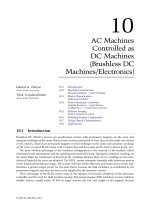
where the eigenvalues are complex with zero real part; thus, for this substructure the phase trajectories
are circles, as shown in Fig. 8.1 and the system is marginally stable. The second substructure, which is

© 2002 by CRC Press LLC


FIGURE 8.1

Phase-plane description corresponding to substructures I and II.

referred as substructure II, is given by

˙
 x1 = x2

˙
 x 2 = +K ⋅ x 1

(8.2)

In this case the eigenvalues are real and with opposite sign; the corresponding phase trajectories are
shown in Fig. 8.1 and the system is unstable. Only one phase trajectory, namely, x2 = −qx1 ( q = K ),
converges toward the origin, whereas all other trajectories are divergent.
Divide the phase-plane in two regions, as shown in Fig. 8.2; accordingly, at each region is associated
one of the two substructures as follows:
Region I:
Region II:

x1 · (x2 + cx1) < 0 ⇒ Substructure I
x1 · (x2 + cx1) > 0 ⇒ Substructure II

where c is lower than q. The switching boundaries are the x2 axis and the line x2 + cx1 = 0. The system
structure changes whenever the system representative point (RP) enters a region defined by the switching
boundaries. The important property of the phase trajectories of both substructures is that, in the vicinity
of the switching line x2 + cx1 = 0, they converge to the switching line. The immediate consequence of
this property is that, once the RP hits the switching line, the control law ensures that the RP does not
move away from the switching line. Figure 8.2a shows a typical overall trajectory starting from an arbitrary
initial condition P0 (x10, x20): after the intervals corresponding to trajectories P0 – P1 (substructure I) and
P1 – P2 (substructure II), the final state evolution lies on the switching line (in the hypothesis of ideal

infinite frequency commutations between the two substructures).
This motion of the system RP along a trajectory, on which the structure of the system changes and
which is not part of any of the substructure trajectories, is called the sliding mode, and the switching line
x2 + cx1 = 0 is called the sliding line. When sliding mode exists, the resultant system performance is
completely different from that dictated by any of the substructures of the VSS and can be, under particular
conditions, made independent of the properties of the substructures employed and dependent only on

© 2002 by CRC Press LLC


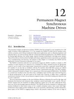
FIGURE 8.2
mode.

Sliding regime in VSS. (a) Ideal switching line; (b) switching line with hysteresis; (c) unstable sliding

the control law (in this example the boundary x2 + cx1 = 0). In this case, for example, the dynamic is of
the first order with a time constant equal to 1/c.
The independence of the closed-loop dynamics on the parameters of each substructure is not usually
true for more complex systems, but even in these cases it has been proved that the sliding-mode control
maintains good robustness compared with other control techniques. For higher-order systems, the control

© 2002 by CRC Press LLC


rule can be written in the following way:
N

s = f ( x 1 ,…, x N ) =

∑c x

i i

= 0

(8.3)

i=1

where N is the system order and xi are the state variables. Note that the choice of using a linear combination of state variable in Eq. (8.3) is only one possible solution, which results in a particularly simple
implementation in SMPS applications.
When the switching boundary is not ideal, i.e., the commutation frequency between the two substructures is finite, then the overall system trajectory is as shown in Fig. 8.2b. Of course, the width of the
hysteresis around the switching line determines the switching frequency between the two substructures.
Following this simple example and looking at the Figs. 8.1 and 8.2, it is easy to understand that the
conditions for realizing a sliding-mode control are:
• Existence condition: The trajectories of the two substructures are directed toward the sliding line
when they are close to it.
• Hitting condition: Whatever the initial conditions, the system trajectories must reach the sliding
line.
• Stability condition: The evolution of the system under sliding mode should be directed to a stable
point. In Fig. 8.2b the system in sliding mode goes to the origin of the system, that is, a stable
point. But if the sliding line were the following:
Region I: x1 · (x2 + cx1) < 0 ⇒ Substructure I
Region II: x1 · (x2 + cx1) > 0 ⇒ Substructure II
where c < 0, then the system trajectories would have been as shown in Fig. 8.2c. In this case, the resulting
state trajectory still follows the sliding line, but it goes to infinity and the system is therefore unstable.
The approach to more complex systems cannot be expressed only with graphical considerations, and
a mathematical approach should be introduced, as reported below.

8.3 Basics of Sliding-Mode Theory

Consider the following general system with scalar control [1, 2]:

˙
x = f ( x, t, u )

(8.4)

where x is a column vector and f is a function vector, both of dimension N, and u is an element that can
influence the system motion (control input). Consider that the function vector f is discontinuous on a
surface σ (x, t) = 0. Thus, one can write:
+

+

 f ( x, t, u )
f ( x, t, u ) =  −
−
 f ( x, t, u )

for

s→0

+

for

s→0

−

(8.5)

where the scalar discontinuous input u is given by
+

u
u =  −
u

for

s(x) > 0

for

s(x) < 0

The system is in sliding mode if its representative point moves on the sliding surface σ (x, t) = 0.

© 2002 by CRC Press LLC

(8.6)


Existence Condition
For a sliding mode to exist, the phase trajectories of the two substructures corresponding to the two different
values of the vector function f must be directed toward the sliding surface σ (x, t) = 0 in a small region
close to the surface itself. In other words, approaching the sliding surface from points where σ < 0, the
−

corresponding state velocity vector f must be directed toward the sliding surface, and the same must
happen when points above the surface (σ > 0) are considered, for which the corresponding state velocity
+
+
−
vector is f . Indicating with subscript N the components of state velocity vectors f and f orthogonal
to the sliding surface one can write:
+

+

lim f N < 0
s→o

lim ∇s ⋅ f < 0

+

lim f > 0
s→o

−

s →o

⇒

−
N

+

(8.7)

−

lim ∇s ⋅ f > 0
s→o

−

where ∇σ is the gradient of surface σ. Since

ds
------ =
dt

N

∂s dx i

∑ ------ ------∂x dt

= ∇s ⋅ f

(8.8)

i

i=1

the existence condition of the sliding mode becomes

lim ds < 0
-----+
dt

s→o

ds
lim ------ > 0
− dt
s→o

ds
⇒ lim s ------ < 0
dt
s →o

(8.9)

When the inequality given by Eq. (8.9) holds in the entire state space and not only in an infinitesimal
region around the sliding surface, then this condition is also a sufficient condition that the system will
reach the sliding surface.

Hitting Conditions
+

−

+

−

Let [x ] and [x ] be the steady-state RPs corresponding to the inputs u and u Eq. (8.6), respectively.
Then a simple sufficient condition, that will be used later in the application of the sliding mode control
to switch-mode power supplies, for reaching the sliding surface is given by:
+

[ x ] ∈ s ( x ) < 0,

−

[x ] ∈ s(x) > 0

(8.10)

In other words, if the steady-state point for one substructure belongs to the region of the phase space
reserved to the other substructure, then sooner or later the system RP will hit the sliding surface.

System Description in Sliding Mode: Equivalent Control
The next focus of interest in the analysis of VSS is the behavior of the system operating in sliding regime.
Consider here a particular class of systems that are linear with the control input, i.e.,

˙
x = f ( x, t ) + B ( x, t )u
N

N

1

where x ∈ ℜ , f and B ∈ ℑ , u ∈ ℜ .

© 2002 by CRC Press LLC

(8.11)


The scalar control input u is discontinuous on the sliding surface σ (x, t) = 0, as shown in Eq. (8.6),
whereas f and B are continuous function vectors. Under sliding mode control, the system trajectories
stay on the sliding surface, hence:

s ( x, t ) = 0 ⇒ s ( x, t ) = 0
ds
˙
s ( x, t ) = ------ =
dt

N

∂s dx i

∑ ------ ------∂x dt
i =1

˙
˙
= ∇s ⋅ x = Gx

(8.12)

(8.13)

i

where G is a 1 by N matrix whose elements are the derivatives of the sliding surface with respect to the
state variables. By using Eqs. (8.11) and (8.13),

˙
Gx = Gf ( x, t ) + GB ( x, t )u eq = 0

(8.14)

where the control input u was substituted by an equivalent control ueq that represents an equivalent
continuous control input that maintains the system evolution on the sliding surface. On the assumption
−1
that [GB] exists, from Eq. (8.14) one can derive the expression for the equivalent control:
−1

u eq = − ( GB ) Gf ( x, t )

(8.15)

Finally, by substituting this expression into Eq. (8.11),
−1
˙
x = [ I – B ( GB ) G ]f ( x, t )

(8.16)

Equation (8.16) describes the system motion under sliding-mode control. It is important to note that
−1
the matrix I – B ( GB ) G is less than full rank. This is because, under sliding regime, the system motion
is constrained to be on the sliding surface. As a consequence, the equivalent system described by Eq. (8.16)
is of order N − 1. This equivalent control description of a VSS in sliding regime is valid, of course, also
for multiple control inputs. For details, see Refs. 1 and 2.

Stability
Analyzing the system behavior in the phase-plane for the second-order system, it was found that the
system stability is guaranteed if its trajectory, in sliding regime, is directed toward a stable operating
point. For higher-order systems, a direct view of the phase space is not feasible and one must prove
system stability through mathematical tools. First consider a simple linear system with scalar control in
the following canonical form:

˙
i = 1, 2, …,N – 1
 x i = x i+1

N

˙
a Nj x j + bu
 xN =

j=1

∑

(8.17)

and
N

N

s ( x, t ) =

∑
i =1

ci xi =

i−1

d x
c i ------------1 = 0
i−1
dt
i =1

∑

(8.18)

The latter equation completely defines the system dynamic in sliding regime. Moreover, in this case
the system dynamic in sliding mode depends only on the sliding surface coefficients ci, leading to a system
behavior that is completely different from those given by the substructures defined by the two control

© 2002 by CRC Press LLC

+

−

input values u and u . This is a highly desirable situation because the system dynamic can be directly
determined by a proper ci selection. Unfortunately, in the application to DC-DC converters this is possible
only for the buck topology, whereas for other converters, state derivatives are not only difficult to measure,
but also discontinuous. Therefore, we are obliged to select system states that are measurable, physical,
and continuous variables. In this general case, the system stability in sliding mode can be analyzed by
using the equivalent control method Eq. (8.16).

8.4 Application of Sliding-Mode Control to DC-DC
Converters—Basic Principle
The general sliding-mode control scheme of DC-DC converters is shown in Fig. 8.3. Ug and uo are input
and output voltages, respectively, while iLi and uCj (i = 1 ÷ r, j = r + 1 ÷ N − 1) are the internal state
variables of the converter (inductor currents and capacitor voltages). Switch S accounts for the system
nonlinearity and indicates that the converter may assume only two linear subtopologies, each associated
to one switch status. All DC-DC converters having this property (including all single-switch topologies,
plus push-pull, half and two-level full-bridge converters) are represented by the equivalent scheme of
Fig. 8.3. The above condition also implies that the sliding-mode control presented here is valid only for
continuous conduction mode (CCM) of operation.
In the scheme of Fig. 8.3, according to the general sliding-mode control theory, all state variables are
sensed, and the corresponding errors (defined by difference to the steady-state values) are multiplied by
proper gains ci and added together to form the sliding function σ. Then, hysteretic block HC maintains
this function near zero, so that
N

s =

∑c e

i i

= 0

(8.19)

i=1

Observe that Eq. (8.19) represents a hyperplane in the state error space, passing through the origin. Each
of the two regions separated by this plane is associated, by block HC, to one converter sub structure. If one
assumes (existence condition of the sliding mode) that the state trajectories near the surface, in both regions,

FIGURE 8.3

Principle scheme of a SM controller applied to DC-DC converters.

© 2002 by CRC Press LLC


are directed toward the sliding plane, the system state can be enforced to remain near (lie on) the sliding
plane by proper operation of the converter switch(es).
Sliding-mode controller design requires only a proper selection of the sliding surface Eq. (8.19), i.e.,
of coefficients ci, to ensure existence, hitting, and stability conditions. From a practical point of view,
selection of the sliding surface is not difficult if second-order converters are considered. In this case, in
fact, the above conditions can be verified by simple graphical techniques. Instead, for higher-order
converters, like Cúk and SEPIC, the more general approach outlined in Section 8.5 must be used.
One of the major problem of the general scheme of Fig. 8.3 is that inductor current and capacitor

voltage references are difficult to evaluate, because they generally depend on load power demand, supply
voltage, and load voltage. This is true for all basic topologies, except the buck converter, whose dynamic
equations can be expressed in canonical form Eq. (8.17). Thus, for all converters, except the buck topology,
some provisions are needed for the estimation of such references, strongly affecting the closed-loop dynamics, as discussed in the following sections.

8.5 Sliding-Mode Control of Buck DC-DC Converters
It was already mentioned that one of the most important features of the sliding-mode regimes in VSS is
the ability to achieve responses that are independent of system parameters, the only constraint being the
canonical form description of the system. From this point of view, the buck DC-DC converter is particularly suitable for the application of the sliding-mode control, because its controllable states (output
voltage and its derivative) are all continuous and accessible for measurement.

Phase-Plane Description
The basic buck DC-DC converter topology is shown in Fig. 8.4.
In this case it is more convenient to use a system description, which involves the output error and its
derivative, i.e.,

 x 1 = u o – U o∗


dx 1
du o
iC
 x 2 = ------- = ------- = --dt
dt
C


FIGURE 8.4
positions.

(8.20)

Buck DC-DC converter topology and related substructures corresponding to two different switch

© 2002 by CRC Press LLC


FIGURE 8.5 (a) Phase trajectories of the substructure corresponding to u = 1; (b) Phase trajectories of the substructure corresponding to u = 0; (c) Subsystem trajectories and sliding line in the phase-plane of the buck converter.

The system equations, in terms of state variables x1 and x2 and considering a continuous conduction
mode (CCM) operation can be written as

 x1 = x2
˙

∗

x1 x2 Ug
Uo
˙
 x 2 = − ------ – ------ + ------ u – -----LC RC LC
LC


(8.21)

where u is the discontinuous input, which can assume the values 0 (switch OFF) or 1 (switch ON). In
state-space form:

˙

x = Ax + Bu + D
A =

0
1
1
1 ,
− ------ − -----LC
RC

0

0
B = Ug ,
-----LC

D=

∗

(8.22)

Uo
− -----LC

Practically, the damping factor of this second-order system is less than 1, resulting in complex conjugate
eigenvalues with negative real part. The phase trajectories corresponding to the substructure u = 1 are shown
in Fig. 8.5a for different values of the initial conditions. The equilibrium point for this substructure is
∗
xleq = Ug − U o and x2eq = 0. Instead, with u = 0 the corresponding phase trajectories are reported in

∗
Fig. 8.5b and the equilibrium point for this second substructure is xleq = − U o and x2eq = 0.
Note that the real structure of Fig. 8.5b has a physical limitation due to the rectifying characteristic of
the freewheeling diode. In fact, when the switch S is OFF, the inductor current can assume only nonnegative values. In particular, when iL goes to zero it remains zero and the output capacitor discharge
goes exponentially to zero. This situation corresponds to the discontinuous-conduction mode (DCM)
and it poses a constraint on the state variables. In other words, part of the phase-plane does not correspond
to possible physical states of the system and so need not be analyzed. The boundary of this region can
be derived from the constraint iL = 0 and is given by the equation:
∗

Uo
1
x 2 = − ------ x 1 – -----RC
RC

(8.23)

which corresponds to the straight line with a negative slope equal to −1/RC and passing through the
∗
∗
point (−U o , 0) shown in dashed line in Fig. 8.5b. In the same figure, the line x 1 = – U o is also reported,
which defines another not physically accessible region of the phase-plane, i.e., the region in which uo < 0.

© 2002 by CRC Press LLC


Selection of the Sliding Line
It is convenient to select the sliding surface as a linear combination of the state variables because the
results are very simple to implement in the real control system and because it allows the use of the
equivalent control method to describe the system dynamic in sliding mode. Thus, we can write:

T

s ( x ) = c1 x1 + x2 = C x = 0

(8.24)

T

where C = [c1, 1] is the vector of sliding surface coefficients which corresponds to G in Eq. (8.13), and
coefficient c2 was set to 1 without loss of generality.
As shown in Fig. 8.5c, this equation describes a line in the phase-plane passing through the origin,
which represents the stable operating point for this converter (zero output voltage error and its derivative).
By using Eq. (8.21), Eq. (8.24) becomes

˙
s ( x ) = c1 x1 + x1 = 0

(8.25)

which completely describes the system dynamic in sliding mode. Thus, if existence and reaching conditions of the sliding mode are satisfied, a stable system is obtained by choosing a positive value for c1.
Figure 8.5c reveals the great potentialities of the phase-plane representation for second-order systems.
In fact, a direct inspection of Fig. 8.5c shows that if we choose the following control law:

0
u = 
1

for
for

s(x) > 0
s(x) < 0

(8.26)

then both existence and reaching conditions are satisfied, at least in a small region around the system
equilibrium point. In fact, we can easily see that, using this control law, for both sides of the sliding line
the phase trajectories of the corresponding substructures are directed toward the sliding line (at least in
a small region around the origin). Moreover, the equilibrium point for the substructure corresponding
to u = 0 belongs to the region of the phase-plane relative to the other substructure, and vice versa, thus
ensuring the reachability of the sliding line from any allowed initial state condition. From Eq. (8.5) it is
easy to see that the output voltage dynamics in sliding mode is simply given by a first-order system with
time constant equal to 1/c1. Typical waveforms with c1 = 0.8/RC are reported in Fig. 8.6.

FIGURE 8.6 (a) Phase trajectories for two different initial conditions (c1 = 0.8/RC); (b) Time responses of normalized output voltage uoN and normalized inductor current iLN (c1 = 0.8/RC) (initial conditions in P1).

© 2002 by CRC Press LLC


Existence Condition
Let us analyze more precisely the existence of the sliding regime for the buck converter. From the slidingmode theory, the conditions for the sliding regime to exist are (see Eq. 8.9):
T

T

+

T

 C Ax + C Bu + C D < 0

˙
s(x) =  T
T
−
T
 C Ax + C Bu + C D > 0

for

0 < s(x) < x

for

−x < s ( x ) < 0

(8.27)

where ξ is an arbitrary small positive quantity. Using Eqs. (8.22) and (8.24) these inequalities become
∗

Uo
1
1
 l 1 ( x ) =  c 1 – ------  x 2 – ------ x 1 – ------ < 0

LC
LC
RC



∗
Ug – Uo

1
1
l 2 ( x ) =  c 1 – ------  x 2 – ------ x 1 + ----------------- > 0


LC
LC
RC


for

0 < s(x) < x

for

−x < s ( x ) < 0

Equations λ1(x) = 0 and λ2(x) = 0 define two lines in the phase-plane with the same slope passing
∗
∗
through points (−U o , 0) and (Ug − U o , 0), respectively. The regions of existence of the sliding mode
are depicted in Fig. 8.7 for two different situations: (1) c1 > 1/RC, and (2) c1 < 1/RC. As we can see,
the increase of c1 value causes a reduction of sliding-mode existence region. Remember that the sliding
line coefficient c1 determines also the system dynamic response in sliding mode, since the system
dynamic response results are of first order with a time constant τ = 1/c1. Thus, high response speeds,
i.e., τ < RC, limit the existence region of the sliding mode. This can cause overshoots and ringing

during transients.
To better understand this concept, let us take a look to some simulation results. Figure 8.7 shows the
phase trajectories of a buck converter with sliding-mode control for two different c1 values where the
∗
initial condition is in (−U o , 0): when the slope of the sliding line becomes too high, as shown in Fig. 8.7a,
the system RP hits first the sliding line at a point outside the region of the existence of the sliding mode.
As a consequence, the switch remains in a fixed position (open in this case) until the RP hits the sliding
line again, now in a region where the existence condition is satisfied.

σ(x) = 0

λ1

x2
λ1

x2

λ2

σ(x) = 0
u=0

u=1
λ2

u=0

0

*
Uo

x1

0

*
Uo

Ug

*
Uo

Ug

*
Uo

u=1

iL = 0

a)

FIGURE 8.7

iL = 0

b)

Regions of existence of the sliding mode in the phase-plane: (a) c1 > 1/RC; (b) c1 < 1/RC.

© 2002 by CRC Press LLC

x1


FIGURE 8.8 Time responses of normalized inductor current iLN (a) and normalized output voltage uoN (b) at
different c1 values (k = c1RC).

The time responses of the normalized inductor current iLN and output voltage uoN for different c1 values
are reported in Fig. 8.8a and b respectively (iLN = iL/Io, uoN = uo /Uo). Note that with c1 = 1/RC neither the
inductor current nor the output voltage has overshot during start-up.

Current Limitation
As we have seen from Fig. 8.8b, a fast output voltage dynamic calls for overshoots in the inductor current
iL. In fact, the first part of the transient response depends on the system parameters, and only when the
system RP hits the sliding line at a point belonging to the existence region is the system dynamic dictated
by the sliding equation (for the buck converter it is actually independent of the converter parameters
and dependent only on the sliding coefficient c1). The large inductor current could not be tolerated by
the converter devices for two reasons: it can cause the inductor core to saturate with consequent even
high-peak current value or can be simply greater than the maximum allowed switch current. Thus, it is
convenient to introduce into the controller a protection circuit that prevents the inductor current from
reaching dangerous values. This feature can be easily incorporated into the sliding-mode controller by
a suitable modification of the sliding line. For example, in the case of buck converters, to keep constant
the inductor current we have to force the system RP on the line:
∗

I Lmax U o
1
x 2 = − ------ x 1 + ---------- – -----RC
C
RC

(8.28)

Thus, the global sliding line consists of two pieces:
∗
 x1
Uo
1
 ------ + x 2 – ---  I Lmax – ----- 
s ′ ( x ) =  RC
C
R
c x + x
2
 1 1

for

i L > I Lmax

for

i L < I Lmax

(8.29)

The phase plane trajectories for a buck converter with inductor current limitation and with c1 = 2/RC
are shown in Fig. 8.9, and the corresponding normalized inductor current transient behavior is shown
in Fig. 8.10. It is interesting to note that Eq. (8.29) gives an explanation of why the fastest response

© 2002 by CRC Press LLC


FIGURE 8.9

Phase trajectories for a buck converter with inductor current limitation (c1 = 2/RC).

FIGURE 8.10 Time response of normalized inductor current iLN of a buck converter with current limitation
(c1 = 2/RC).
∗

without overshoots is obtained for c1 = 1/RC. In fact, if c1 = 1/RC and ILmax = U o /R the two pieces of the
∗
sliding line σ ′ become a single line and thus the inductor current reaches its steady-state value U o /R
without overshoot.

8.6 Extension to Boost and Buck–Boost DC-DC Converters
For boost as well as buck–boost DC-DC converters, the derivative of the output voltage turns out to be
a discontinuous variable, and we cannot express the system in canonical form as was done for the buck
converter. Following the general scheme of Fig. 8.3, the inductor current and output voltage errors are
chosen as state variables, i.e.,
∗

 x1 = i – I


∗
 x2 = uo – Uo

(8.30)

∗

where the current reference I depends on the converter operating point (output power and input
voltage). Choosing the same control law Eq. (8.26) of the buck converter, together with the following
sliding line:
T

s ( x ) = x 1 + gx 2 = C x = 0

© 2002 by CRC Press LLC

(8.31)


FIGURE 8.11

Boost converter with sliding-mode control.

it can be easily seen [13] that both existence and reaching conditions are satisfied (the former at least in
a small region enclosing the origin) as long as

RC U g
- g < ------ -----∗
L Uo

(8.32)

∗

for both converters. However, current reference signal I is not usually available in practice, and some
alternative techniques for its estimation are needed. One possible solution is to derive this reference signal
directly from the inductor current by using a low-pass filter, as shown in Fig. 8.11. This estimation clearly
affects the dynamic behavior of the sliding-mode control. To understand the closed-loop dynamics of
this approach, we need to include the additional state variable introduced by the low-pass filter, i.e.,
∗

di
1 ∗ 1
------ = − -- i + -- i
dt
t
t

(8.33)

Taking into account the boost converter, we can represent the overall system, choosing as state variables:

 x1 = i

∗
 x2 = uo – Uo

∗
 x3 = i
˙

x = Ax + Bu + D
0

(8.34)

(8.35)

0
0
1
A = 0 − ------ 0 ,
RC
1
1
-0
− -t
t

© 2002 by CRC Press LLC

uo
− ---L
B= i ,
--C
0

Ug
----L
D=

∗

Uo
− -----RC
0


The sliding line becomes a sliding surface in the phase space:
T

s ( x ) = x 1 + gx 2 – x 3 = C x = 0

(8.36)

T

where C = [1, g, −1] is the vector of the sliding surface coefficients and x1 − x3 represents now the
inductor current error. Fortunately, the existence conditions analysis for the system Eq. (8.35) leads to
the same constraint (8.32), which can be derived without accounting for the low-pass filter dynamic
[13]. However, unlike the buck converter, Eq. (8.32) does not directly give information on the system
stability and on the possible values of filter time constant τ.

Stability Analysis
In the following, a procedure similar to the equivalent control method is used to derive a suitable small
signal model for the system Eq. (8.35) in sliding mode. The starting point is the small-signal state space
averaged model of the boost converter [3]:

˙
ˆ
ˆ

ˆ
ˆ
x = Ax + Bu g + Cd
D′
− ----- 0
L
1
A = D′ − ------ 0 ,
----C
RC
1
1
-0
− -t
t
0

T

1
-L
B=
,
0
0

(8.37)

1
-L

Ug
D = ----1
D′ − ------------D′RC
0

∗ T

ˆ
ˆ ˆ ˆ
where x = [ x 1 , x 2 , x 3 ] = [ ˆ, u o , ˆ ] and D′ = 1 − D. In Eq. (8.37), the dynamic equation of the lowi ˆ i
pass filter Eq. (8.33) was added to the original boost equations. From the sliding surface definition we
can write:
∗
∗
T
ˆ ˆ∗
ˆ
ˆ
s ( x ) = ( i – i ) + g ( u o – U o ) = i – i + gu o = C x

(8.38)

T

where C = [1, g, −1] and the steady-state values X of the state variables coincide with the corresponding
∗
reference values X . Now, if the system is in sliding regime, we can write

˙
T˙

ˆ
s(x) = 0 ⇒ s(x) = C x = 0

(8.39)

From Eqs. (8.37) and (8.39) we can derive an expression for the duty-cycle perturbation as a function
of the state variables and the input, which, substituted into Eq. (8.37), yields:

˙
ˆ
ˆ
ˆ
x = A′ x + B′ u g

(8.40)

In Eq. (8.40), which represents a third-order system, one equation (for example, the last one corresponding to the variable x3) is redundant and can be eliminated by using the equation σ = 0. The result is the

© 2002 by CRC Press LLC


following second-order system:

˙
ˆ
ˆ
ˆ
x = AT x + BT ug ,

1

A T = -k

gD′
− -------C

2 1
g  ------ – --
 RC t

D′
----C

1 gL
------  -------- – 2
RC  D′t 

,

ˆ
ˆ ˆ
x = [ x1 , x2 ]

–g
1
B T = ----------------  
kD′RC  1 

T

(8.41)

where

gL
k = 1 – ------------D′RC

Equation (8.41) completely describe the system behavior under sliding mode control. Moreover, they
can be used to derive closed-loop transfer functions like output impedance and audiosusceptibility, which
allows meaningful comparison with other control techniques. As far as system stability is concerned, by
imposing positive values for the coefficients of the characteristic polynomial we obtain

RCD′
0 < g < g crit = ------------L

(8.42)

and

L
1
t > t crit = ----------- ⋅ --------------------2
2
D′ R 1 + ----------RD′g

(8.43)

It is interesting to note that constraint (8.42) coincides with the existence condition given by (8.32).
As an example of application of the discussed analysis, Fig. 8.12 reports the converter audiosusceptibility and output impedance predicted by the model and experimentally measured in a boost converter
propotype [13] with the following parameters: Ug = 24 V, Uo = 48 V, Po = 50 W, fs = 50 kHz, L = 570 µH,
C = 22 µF, τ = 0.4 ms, g = 0.35. With this value of sliding coefficient g, the stability analysis shows that

the filter time constant τ must be greater than 38 µs for stable operation. Moreover, the chosen value of
400 µs guarantees no output voltage overshoots during transient conditions, as depicted in Fig. 8.13,
which reports simulated waveforms of the startup of the boost converter where the output voltage was
precharged at the input voltage value.

FIGURE 8.12

Comparison between model forecast and experimental results: (a) open loop; (b) closed loop.

© 2002 by CRC Press LLC


TABLE 8.1

Values of τcrit and gcrit for Boost and Buck–Boost Topologies
Boost

Buck–Boost

gcrit

RCD′
------------L

RC D′
------ ----- L D

τcrit

L

1
----------- ⋅ --------------------2
2
D′ R 1 + -----------RD′g

L
-----------------------------------------------2
L
D′
------- R + ( 2 – D′ ) -----D
RC

FIGURE 8.13 Output voltage and inductor current at startup of a boost converter (output capacitor precharged
at input voltage).

The same stability analysis can be applied also to buck–boost converters. As a result, the critical value
for the low-pass filter time constant τcrit and gcrit are given in Table 8.1.

8.7 Extension to Cúk and SEPIC DC-DC Converters
As a general approach to high-order converters like Cúk and SEPIC, a sliding function can be built
N
as a linear combination of all state variable errors xi, i.e., s ( x ) = Σ i=1 c i x i , as depicted in Fig. 8.3.
This general approach, although interesting in theory, is not practical. In fact, it requires sensing of
too many state variables with an unacceptable increase of complexity as compared with such standard
control techniques as current-mode control. However, for Cúk and SEPIC converters a reduced-order
sliding-mode control can be used with satisfactory performances with respect to standard control
techniques [9–11]. In this case, some sliding coefficients are set to zero. In particular, for Cúk and
SEPIC converters, the sensing of only output voltage and input inductor current was proposed and
the current reference signal was obtained, as for the boost and buck–boost converter, by using a lowpass filter. Taking the SEPIC converter as an example, the resulting scheme with reduced-order
implementation is reported in Fig. 8.14. Of course, the same scheme can be applied to Cúk converters

as well.
To give design criteria for selection of sliding-mode controller parameters, the system must be represented in a suitable mathematical form. To this purpose, the converter equations related to the two
subtopologies corresponding to the switch status are written as

˙
v = A on v + F on

(8.44)

˙
v = A off v + F off

© 2002 by CRC Press LLC

switch on,
switch off,

(8.45)


i1
+
Ug

+

L1
S

u1

−

D

C1

L2

C2

+
u2

R

−
1:n
L.P.F

I*
1

+

−
xi

+
xu
H1

Ci

U*
2
−

Cu

+

FIGURE 8.14

SEPIC converter with sliding-mode control.
T

where v = [i1, i2, u1, u2] is the state variable vector. These equations are combined in the following form
(VSS)

˙
v = Av + Bu + F,

(8.46)

where u is the discontinuous variable corresponding to the switch status and matrices A, B, F are given by

A = Aoff,

F = Foff,

(8.47)

B = (Aon − Aoff )v + (Fon − Foff )

(8.48)
∗

It is convenient to write the system Eq. (8.47) in terms of state variables error xi, where x = v − V ,
∗
∗ ∗
∗ T
∗
being V = [ I 1, I 2, U 1, U 2] the vector of state variable references. Accordingly, system equations become

˙
x = Ax + Bu + G,

(8.49)

∗

where G = AV + F.

Existence Condition
Assuming that the switch is kept on when σ is negative and off when σ is positive, we may express the
existence condition in the form (see Eq. 8.9):

∂s
T
T

------ = C Ax + C G < 0
∂t
∂s
T
T
T
------ = C Ax + C B + C G > 0
∂t

0(8.50)
−x < s < 0,

where ξ is an arbitrary small positive quantity. Inequalities (8.50) are useful only if state variable errors
xi are bounded; otherwise, (8.50) must be analyzed under small-signal assumption. In this latter case,
satisfying (8.50) means enforcing the existence condition in a small volume around the operating point,
and this is equivalent to ensuring the stability condition as demonstrated in Ref. 13.

Hitting Condition
If sliding mode exists, a sufficient hitting condition is
T

C A4 ≤ 0

© 2002 by CRC Press LLC

(8.51)


FIGURE 8.15

[13].

Root locus of closed-loop system for variation of low-pass filter time constant of the SEPIC converter

where A4 is the fourth column of matrix A [1, 2]. This yields the following constraint

cu
ci
– ------- – ----------- ≤ 0
nL 1 R L C 2

(8.52)

where ci and cu are the sliding line coefficients for the input current and output voltage errors, respectively,
and n is the ratio between the second and the primary transformer windings.

Stability Condition
This issue must be addressed taking into account the effect of the time constant τ of the low-pass filter
needed to extract the inductor current reference signal. To this purpose the small-signal analysis carried
out for the sliding-mode control of boost converters can be generalized [13]. This can be used to derive
useful design hints for the selection of sliding surface coefficients and filter time constants. As an example,
from the small signal model in sliding mode, similar to (8.41), the root locus of closed-loop system
eigenvalues can be plotted as a function of the low-pass filter time constant as shown in Fig. 8.15 in the
case of a SEPIC converter [11]. Note that the system become unstable for low value of time constant τ.
A similar analysis can be applied to Cúk converters as well.

8.8 General-Purpose Sliding-Mode Control Implementation
Compared to the current control, the sliding-mode approach has some aspects that still must be improved.
The first problem arises from the fact that the switching frequency depends on the rate of change of
function σ and on the amplitude of the hysteresis band. Since σ is a linear combination of state-variable

errors, it depends on actual converter currents and voltages, and its behavior may be difficult to predict.
This can be unacceptable if the range of variation becomes too high. One possible solution of the problem
related to the switching frequency variations is the implementation of a variable hysteresis band, for
example, using a PLL (phase locked loop). Another simple approach is to inject a suitable constantfrequency signal w into the sliding function as shown in Fig. 8.16 [10]. If, in the steady state, the amplitude
of w is predominant in σf , then a commutation occurs at any cycle of w. This also allows converter
synchronization to an external trigger. Instead, under dynamic conditions, error terms xi and xu increase,
w is overridden, and the system retains the excellent dynamic response of the sliding mode. Simulated
waveforms of ramp w, and σPI, σf signals are reported in Fig. 8.17.
The selection of the ramp signal w amplitude is worthy of further discussion. In fact, it should be
selected by taking into account the slope of function σPI and the hysteresis band amplitude, so that
function σf hits the lower part of the hysteresis band at the end of the ramp, causing the commutation.
From the analysis of the waveform shown in Fig. 8.17, we can find that the slope Se of the external ramp

© 2002 by CRC Press LLC


FIGURE 8.16 Reduced-order sliding-mode controller with inductor current limitation, constant switching frequency,
and no output voltage steady-state error.
[mV]
200

w

Se

0
-200
200

Sr

σPI

0
-200
200

σf

0

∆B

-200
0

FIGURE 8.17

20

40

60

80

[ms]

Simulated waveforms of ramp w, and σPI, σf signals.

must satisfy the following inequality

∆B
S e > ------- – S r
dT s

(8.53)

where ∆B represents the hysteresis band amplitude and Sr is the slope of function σPI during the switch
on-time. Note that, in the presence of an external ramp, signal σPI must have a nonzero average value to
accommodate the desired converter duty cycle (see Fig. 8.17). Of course, a triangular disturbing signal
w is not the only waveform that can used. A pulse signal has been used alternatively as reported in Ref. 12.

© 2002 by CRC Press LLC


The second problem derives from a possible steady state error on the output voltage. In fact, when the
inductor current reference is evaluated using a low-pass filter, then the current error leads naturally to
zero average value in steady state. Thus, if the sliding function, due to the hysteretic control or due to
the added ramp signal w, has nonzero average value, a steady-state output voltage error necessarily
appears. This problem can be solved by introducing a PI action on sliding function to eliminate its DC
value (see Fig. 8.16). In practice, the integral action of this regulator is enabled only when the system is
on the sliding surface; in this way, the system behavior during large transients, when σ can have values
far from zero, is not affected, thus maintaining the large-signal dynamic characteristics of sliding-mode
control. A general-purpose sliding-mode controller scheme that includes the aforementioned improvements, together with reduced-order implementation in the case of Cúk and SEPIC converters and a
possible implementation of current limitation by means of another hysteretic comparator and an AND
port, is reported in Fig. 8.16. Experimental results of this scheme are reported in Refs. 10 and 11.

8.9 Conclusions
Control techniques of VSS find a natural application to SMPS, since they inherently show variable
structure properties as a result of the conversion process and switch modulation. Thus, the sliding-mode

control represents a powerful tool to enhance performance of power converters. Sliding-mode control is
able to ensure system stability even for large supply and load variations, good dynamic response, and
simple implementation, even for high-order converters. These features make this control technique a
valid alternative to standard control approaches.
The application of the sliding-mode control technique to DC-DC converters is the focus of this chapter.
The application to buck converters is discussed in detail, whereas for the extension of this control technique
to boost, buck–boost, Cúk, and SEPIC converters only some design guidelines are given. Finally, such
improvements as current limitation, constant switching frequency, and output voltage steady-state error
cancellation are outlined. This control approach can also be effectively used in other applications, not
discussed here, such as inverters [14, 18], power factor controllers [16], and AC power supplies [17].

References
1. V. I. Utkin, Sliding Modes and Their Application in Variable Structure Systems, MIR Publishers,
Moscow, 1978.
2. U. Itkis, Control Systems of Variable Structure, John Wiley & Sons, New York, 1976.
3. R. D. Middlebrook and S. Cuk, Advances in Switched-Mode Power Conversion, Vol. I and II, TESLAco,
Pasadena, CA, 1983, 73–89.
4. R. Redl and N. Sokal, Current-mode control, five different types, used with the three basic classes
of power converters: small-signal AC and large-signal DC characterization, stability requirements,
and implementation of practical circuits, in IEEE-PESC, 1985, 771–785.
5. J. G. Kassakian, M. F. Schlecht, and G. C. Verghese, Principles of Power Electronics, Addison-Wesley,
Reading, MA, 1991.
6. R. Venkataramanan, A. Sabanovic, and S. Cúk, Sliding-mode control of DC-to-DC converters, in
IECON Conf. Proc., 1985, 251–258.
7. B. Nicolas, M. Fadel, and Y. Chéron, Robust control of switched power converters via sliding mode,
ETEP, 6(6), 413–418, 1996.
8. B. Nicolas, M. Fadel, and Y. Chéron, Sliding mode control of DC-to-DC converters with input filter
based on Lyapunov-function approach, in EPE Conf. Proc., 1995, 1.338–1.343.
9. L. Malesani, L. Rossetto, G. Spiazzi, and P. Tenti, Performance optimization of Cúk converters by
sliding-mode control, IEEE Trans. Power Electron., 10(3), 302–309, 1995.

10. P. Mattavelli, L. Rossetto, G. Spiazzi, and P. Tenti, General-purpose sliding-mode controller for
DC/DC converter applications, in Proc. of IEEE Power Electronics Specialists Conf. (PESC), Seattle,
June 1993, 609–615.

© 2002 by CRC Press LLC


11. P. Mattavelli, L. Rossetto, G. Spiazzi, and P. Tenti, Sliding mode control of SEPIC converters, in Proc.
of European Space Power Conf. (ESPC), Graz, August 1993, 173–178.
12. J. Fernando Silva and Sonia S. Paulo, Fixed frequency sliding mode modulator for current mode
PWM inverters, in Power Electronics Specialists Conf. Proc. (PESC), 1993, 623–629.
13. P. Mattavelli, L. Rossetto, and G. Spiazzi, Small-signal analysis of DC-DC converters with sliding
mode control, IEEE Trans. Power Electron., 12(1), 79–86, 1997.
14. N. Sabanovic, A. Sabanovic, and K. Ohnishi, Sliding mode control of three-phase switching converters,
in Proc. of Int. Conf. on Industrial Electronics, Control and Instrumentation (IECON), San Diego, 1992,
319–325.
15. N. Sabanovic-Behlilovic, A. Sabanovic, and T. Ninomiya, PWM in three-phase switching converterssliding mode solution, in Power Electronics Specialists Conference, PESC ’94 Record, 25th Annual IEEE,
Vol. 1, 1994, 560–565.
16. L. Rossetto, G. Spiazzi, B. Fabiano, and C. Licitra, Fast-response high-quality rectifier with sliding
mode control, IEEE Trans. Power Electron., 9(2), 146–152, 1994.
17. L. Malesani, L. Rossetto, G. Spiazzi, and A. Zuccato, An AC power supply with sliding-mode control,
IEEE Ind. Appl. Mag., 2(5), 32–38, 1996.
18. H. Pinheiro, A. S. Martins, and J. R. Pinheiro, A sliding mode controller in single phase voltage
source inverters, in IEEE IECON ’94, 1994, 394–398.
19. H. Sira-Ramirez and M. Rios-Bolivar, Sliding mode control of DC-to-DC power converters via
extended linearization circuits and systems I: fundamental theory and applications, IEEE Transactions
on Circuits and Systems 41(10), 652–661, 1994.

© 2002 by CRC Press LLC