Comparison of the capital asset pricing model and the three factor model in a business cycle: Empirical evidence from the Vietnamese stock market
Bạn đang xem bản rút gọn của tài liệu. Xem và tải ngay bản đầy đủ của tài liệu tại đây (646.28 KB, 13 trang )
VNU Journal of Science: Economics and Business, Vol. 36, No. 2 (2020) 13-25
Original Article
Comparison of the Capital Asset Pricing Model
and the Three-Factor Model in a Business Cycle:
Empirical Evidence from the Vietnamese Stock Market
Luong Tram Anh*
VNU University of Economics and Business, Vietnam National University, Hanoi,
144 Xuan Thuy, Cau Giay, Hanoi, Vietnan
Received 6 November 2019
Revised 09 June 2020; Accepted 15 June 2020
Abstract: Using data from 2010 to 2019, for the first time, the Capital Asset Pricing Model
(CAPM) and the Three-factor Model (TFM) are compared in different contexts of the Vietnamese
economy (recession and recovery). This paper employs four tests including the t-test,
determination coefficient R2, Chow-test and GRS-test to examine the performance of the two
models. Results show the superiority of the TFM over the CAPM in both contexts of the economy,
consistent with Fama and French’s studies. This promises that the TFM can be used to replace the
CAPM in capturing the cost of equity. Another finding is that the two models tend to perform
better in recession than recovery. This study contributes to the literature about asset-pricing models
and their performances in different economic contexts. Moreover, the findings also offer insights
into the use of the CAPM and TFM in developing countries in general and Vietnam, in particular.
Keywords: Capital asset pricing model, three-factor model, business cycle, developing countries.
1. Introduction *
determine the variation in stock returns such as
the APT model, Capital Asset Pricing Model
(CAPM) and Fama-French Three-factor Model
(TFM). One of the most important models is the
CAPM. Being first introduced by Sharpe (1964)
and then developed by Lintner (1965) and
Jensen (1968), the CAPM has become one of
the most popular asset-pricing models that
address the risk-return trade off. Assumptions
of this model are summarized as follows [1]:
1.1. The Capital Asset Pricing Model (CAPM)
and Fama-French Three-Factor Model (TFM)
The return is a fundamental factor that
affects investment decisions on the stock
market. There are many asset-pricing models to
_______
*
Corresponding author.
E-mail address:
/>
13
14
L.T. Anh / VNU Journal of Science: Economics and Business, Vol. 36, No. 2 (2020) 13-25
i) “Mean-variance-efficiency”: All investors
make decisions depending on risk and expected
returns only.
ii) Homogeneity of investor expectations:
All investors have the same beliefs in
investments (the expected values and the
variance of expected returns).
iii) All investors can borrow and lend any
risk-free assets and any risky securities
regardless of the amount they borrow or lend.
iv) Capital markets are perfectly
competitive. No transaction costs and taxes
regardless of investors’ investment and
transactions.
v) All transactions are made at a certain time.
E ( R j R f i j E ( RM ) R f i (1)
Where αi = the intercept of regression,
βi = the slope of regression, εi = the random
error; RM = returns on the market, Rf = freerisk return. In the test of the effectiveness of the
CAPM, Fama and French (1992) observed the
rate of returns on New York Stock Exchange
(NYSE) stocks and concluded that this model
could not explain returns between 1941 and
1990, especially between 1963 and 1990 [2].
Besides the risk premium, they added two other
factors that influenced returns: the size (ME)
and the book-to-market equity (BE/ME) of a
company. Thus, the return was explained by
three factors and the Fama-French model is:
E(Ri) – Rf = αi + βi[E(RM) – Rf] + siSMB +
hiHML + εi (2)
Where βi, si and hi = the slopes in the timeseries regression; εi = mean-zero regression
disturbance; SMB (Small Minus Big) = 1/3
(Small Value + Small Neutral + Small Growth)
- 1/3 (Big Value + Big Neutral + Big Growth)
(This is the average return on three small
portfolios minus the average return on three big
portfolios); HML (High Minus Low) = 1/2
(Small Value + Big Value) - 1/2 (Small Growth
+ Big Growth) (It is the average return on two
value portfolios minus the average return on
two growth portfolios).
While the TFM is increasingly popular in
capturing returns as well as calculating the cost
of equity, the CAPM is still the most prevalent
model in finance. The comparison between the
two models has received a good deal of
attention from researchers.
On the one hand, many studies in different
periods show the superiority of the TFM over
the CAPM. Data from the NYSE, AMEX and
American/Canadian
Stock
Exchange
(NASDAQ) between 1962 and 1989 indicated
“negative conclusions about the roles of beta in
average returns” (Fama and French, 1992) [2].
Research by Fama and French (1993) again
proved the negative relation between size and
average returns, as well as the strong positive
relation between BE/ME and average returns
[3]. Fama and French (1996) reaffirmed this
conclusion when observing data from 1963 to
1993. They formed portfolios based on P/E,
cash flow/price, sales growth and long-term
past returns. Consequently, not only the GRSstatistic rejected the CAPM at the 99 per cent
confidence level, but also the regression
showed large average absolute pricing errors of
the CAPM (three to five times greater than
those of the TFM) [4]. Fama and French (1996)
concluded that the TFM dominated on almost
all portfolios except for portfolios formed on
short-term past returns [4]. Malin and Ahlem
(2007) also tested the two models on the
Toronto Stock Exchange and showed that the
TFM outperforms the CAPM because the
generalized method of moments indicated a
lower intercept of the TFM than the CAPM [5].
Furthermore, the sample determination
coefficient also proved that the Fama-French
model was more reliable. The conclusions of
this study are consistent with Fama and
French’s findings (1992) that firms having a
small size and a great BE/ME ratio seem to gain
higher returns than those having a large size but
a small BE/ME ratio [2]. Billou (2004)
extended the Fama and French’s study by
examining a longer period from 1926 to 2003;
however, the results are slightly different. There
are two tests in this paper: first, tests on 25
portfolios sorted by size and book-to-market
ratio; second, tests on 12 industry portfolios.
While results from 25 portfolios support the
L.T. Anh / VNU Journal of Science: Economics and Business, Vol. 36, No. 2 (2020) 13-25
TFM, results from 12 portfolios show that the
CAPM is better. In conclusion, Billou (2004)
said that the Fama-French factors are firm
specific; and the performance of the two models
based on the type of portfolio grouping [6].
On the other hand, Bartholdy and Peare
(2004) advocated the CAPM over the TFM [7].
This research considers two different market
factors: The Center for Research in Security
Prices (CRSP) Equal-Weighted Index and the
Economy Index. Data was collected from the
NYSE from 1975 to 1996. The sample
determination coefficient of the regression
showed that the CRSP Equal-Weighted Index
provided the best estimating beta based on the
CAPM. In the same way, Grauer and Janmaat
(2009) ran data from 1963 to 2005 on the
NYSE to compare the two models [8]. To
reduce the problem of reduced beta spread, they
used repacked 14 real world datasets from Ken
French’s website in four zero-weight datasets.
Ordinary Least Squares (OLS) regression and
General Least Squares (GLS) regression were
employed to test whether positive slopes of
excess returns on betas were rejected or not. As
a result, in the tests of 14 standard datasets, the
CAPM was supported in only one dataset
compared to none for the TFM. In tests of the
four repackaged datasets, the CAPM was again
better with all positive coefficients (twice
higher than the number of positive coefficients
of the TFM).
Although there are many researches to
discuss the effectiveness of the CAPM and the
Fama-French model, the comparisons are
mainly made over long periods. This has the
potential to lead to inaccurate results because
the performance of a company is significantly
affected by the business environment. Hence,
the intention of this study is to concentrate on
the question whether the CAPM and the TFM
display in different ways in recession and in
recovery. The findings will contribute to the
literature on asset-pricing models. Furthermore,
studies in this field mainly focus on companies
in developed countries; it is necessary to
analyze these markets to know whether the two
models perform in a different way from
15
developed countries or not. I choose Vietnam
because this is a typical developing country
with a high growth rate and is a potential
destination for both foreign and domestic
investors. Identifying a suitable asset-pricing
model for this market is important for making
decisions about adding stocks to investors’
portfolios. The methodology in this study can
be a foundation for future studies to evaluate
the two models in other developing economies.
By updating data until September 2019, this
study will provide comprehensive knowledge as
well as empirical tests on these two models.
1.2. Economic Cycle
The purpose of this research is to compare
the CAPM and the TFM in different business
contexts in Vietnam. Therefore, it is necessary
to review the literature on economic cycles.
An economic cycle (or business cycle) is
alternating periods of recessions and
expansions. It seems to be consistent with
changes in Gross Domestic Product (GDP).
Dow (1998) considered the business cycle in
terms of the capacity rate of growth, which is
“the rate of output growth at which
unemployment tends to remain constant” [9].
Recession looms when the output growth rate
falls below the estimated trend of capacity
growth, and recovery starts when growth
exceeds the capacity growth rate.
However, GDP and unemployment are the
only measures to imply the economic cycle.
There are a number of factors affecting the
output growth rate. Chadha and Warren (2013)
clarified the variation in output by considering
four sets of residuals: labour supply, productive
efficiency, investment and total expenditure
[10]. The Economic Cycle Research Institute
(ECRI) (2015) has a similar view of the
business cycle. There are four variables relating
to the business cycle including employment,
income, productivity and sales. On occasion,
one of these factors can dip, but no recession
will occur despite a negative-output growth.
Recession really occurs when the four measures
all fall together [11].
16
L.T. Anh / VNU Journal of Science: Economics and Business, Vol. 36, No. 2 (2020) 13-25
Knoop (2015) expanded on studies by
Chadha and Warren (2013) and ECRI (2015) by
considering more indicators to describe an
economic cycle, including: Expenditures, Net
exports, Labor market variables, Inflation,
Financial variables and Expectations. Of these,
the unemployment rate and expectations are
lagging countercyclical variables [12]. This is
because when the economy starts to slow down
(or make a recovery), a part of the total labour
force can still get jobs (or be re-added
by companies).
Turning to the length of an economic cycle,
Knoop (2015) concluded that recession and
recovery do not follow a regular pattern. The
length of time of a recession is also different
from that of an expansion [12]. Dow (1998) and
Banerji, Layton and Achuthan (2012) agreed
that recession could be typically shorter than
expansion because an economy tends to take
many years to improve to its previous level
before the recession [9].
This paper is structured as follows: The first
section is the Introduction, reflecting general
understandings about the CAPM and the TFM
and research problems, research aims and the
contribution of this study. The next section
provides information about the background of
this study. The third section explains materials
and methods. The results from three tests on the
two models on the Vietnamese stock market are
presented in the fourth section. The fifth section
summarizes the findings of this paper. The last
section gives recommendations for investors
and financial managers in Vietnam.
Xuan Phuc in dialogue with leaders of
multinational corporations on Viet Nam’s
economy at the World Economic Forum 2019,
the Vietnamese economy has reached a high
growth rate of 7.08%, making it one of the top
growth performers in the region and the world
[14]. Vietnam joined the World Trade
Organization (WTO) in 2007 and became an
official member of the ASEAN Economic
Community (AEC) in 2015, making this market
become more competitive. However, the
Vietnamese economy still has faced many
challenges
with
continuing
domestic
macroeconomic instability, changes in society
and environment issues.
2.2. The Vietnamese Stock Market
Together with the banking system, the stock
market plays important roles in allocating funds
and supporting the liquidity of the economy.
The first stock exchange was launched in 2000
and is known as the Ho Chi Minh City Stock
Exchange (HOSE). This is the biggest stock
exchange in Vietnam. The Vietnam Stock Index
(VN-Index) is the capitalization-weighted index
of all the companies listed on the HOSE. After
19 years of operation, the Vietnamese stock
market has experienced a dramatic development
in both volume and quality. The trading volume
per day on the Vietnamese stock market
increased rapidly from 4.2 million USD in July
2000, to about 120 billion in June 2019 [15].
3. Materials and Methods
3.1. Materials
2. The Background of the Study
2.1. The Vietnamese Economy
The Vietnamese economy started to be
developed from the Doi Moi economic reform
in 1986. Vietnam transformed from one of the
low-income nations with a per capita income
below $100, to a lower-middle-income country
with a per capita income in 2018 of over $2500
[13]. According to Prime Minister Nguyen
For the aims of this study, the monthly
returns of the VN-Index and 97 Vietnamese
companies were collected from January 30,
2010 to September 30, 2019, obtained from
Vndirect Securities Corporation’s website. The
validity and reliability of secondary data refers
to the suitability of data and the reputation of
data sources [16]. In terms of measurement
validity, the sample includes 97 companies in
Forbes’s top 50 listed companies in Vietnam
L.T. Anh / VNU Journal of Science: Economics and Business, Vol. 36, No. 2 (2020) 13-25
between 2010 and 2019. Based on financial
statements audited over five consecutive years,
Forbes considers these companies as leading
companies having typical features of good
Vietnamese firms. Therefore, the data is
relevant and suitable for the purpose of this
study. In terms of reliability, the assessment is
based on the organization providing data and
the data collection technique [16]. The data
studied was collected from Vndirect Securities
Corporation’s website. Vndirect was founded in
2006 and is a reputable financial corporation in
Vietnam. They provide standardized information
about all companies listed on the HOSE. Vndirect
is in the Top 4 companies holding the largest
market share in HOSE [17]. The information on
the Vndirect’s website is updated daily from
companies’ financial reports. Furthermore,
regarding the reliability of results, the data was
collected during approximately a 10-year period
with a sample size of 118. Thus, the number of
observations is sufficient to make statistical
analysis such as doing regression and
undertaking statistical tests. Excel software is
employed for statistical analysis.
3.2. Method
Data collected is separated into two periods:
the recession from January 2010 to December
2012 and the recovery from January 2013 to
September 2019. The reason for splitting is
to test whether the performance of the
two asset-pricing models is influenced by
business contexts.
For the purpose of this study, stocks are
sorted monthly based on market value (ME)
and book-to-market value (BE/ME). The ME
breakpoints are the median of the ME of all
securities studied; and the BE/ME breakpoints
are the 30th and 70th percentiles (Fama and
French, 2015) (Figure 1). As a result, there are
six groups: S/L, S/M, S/H, B/L, B/M, B/H
(Figure 1).
Time-series regressions are used to evaluate
the effectiveness of the CAPM and the TFM.
The change in the VN-Index is used as the
market return (Rm). The three-month
17
Vietnamese Treasury Bill rate is the risk-free
rate of interests (Rf).
Figure 1. Benchmark Portfolios.
Source: Fama and French, 2015 [18].
In this study three measures are concerned
to compare the two models:
Firstly, the t-statistic is employed to test the
hypotheses about intercepts and slopes in each
single regression. The null hypotheses that each
intercept or each slope equals to zero is rejected
if the absolute value of the t-statistic is bigger
than the critical t value at the α/2 level
of significance.
Secondly, the coefficient of determination
(R2) is also used to explain the relationship
between dependent and independent variables
because it implies the explanatory power of
factors in describing average returns. The better
model should have higher R2.
The third measure to evaluate the
performance of the two models is the Chowtest. Due to the ability to test the joint
significance of regression coefficients, the
Chow-test is also employed to test whether a set
of slopes equals to zero in economics. In this
study, the S/L portfolio is considered as the
base category. There are five dummy variables
relating to five portfolios (the S/M, S/H, B/L,
B/M and B/H group). The equation i) of the
CAPM and equation ii) of the TFM are
developed into equation iii) and iv) by adding
dummy variables, respectively. To be simple,
the intercepts of equation iii) and iv) are noted
in terms of i .
L.T. Anh / VNU Journal of Science: Economics and Business, Vol. 36, No. 2 (2020) 13-25
18
portfolio i in period t are jointly normally
distributed each period with
) = 0 and
, and the error terms are serially
uncorrelated (
) = 0) [19]. The GRSstatistic for the regression with T observations,
N portfolios and L independent variables is that
And
Where rp
= the factor mean vector;
the unbiased estimate of the covariance
matrix of the factors; ˆ 0 the least squares
Where XM is excess returns on the market
portfolio over the risk-less portfolio:
X M j E ( RM ) R f .
D1 is dummy variables for the S/M
portfolio: D1 is equal to 1 if the observation
relates to the S/M portfolio, 0 otherwise.
Similarly, D2 , D3 , D4 and D5 are respectively
for the S/H, B/L, B/M, and B/H. i , i and i
are coefficients that represent the extra
overhead returns on the S/M, S/H, B/L, B/M,
B/H portfolio relative to the returns on the S/L
portfolio due to the effect of the market factor,
size factor and BE/ME factor, respectively. To
test for the joint significance of slopes in
equation i) and ii), the null hypothesis of
equation iii) (H0: i 0 and the null hypothesis
of equation iv) (H0: i i i 0 are tested
by an F-test. H0 will be rejected if the value of
the F-statistic is higher than the critical value of
F(k-1, n-k) with k is the number of independent
variables and n is the number of observations
(Dougherty, 2011). This means all factors
contribute to the explanation of returns. In this
case, the greater the F-test, the better the model
performs.
Fourthly, a GRS-test is employed to test
whether the intercepts in equations i) and ii) are
jointly zero or not. Gibbons, Ross and Shanken
(1989) assumed that disturbance terms for
estimator for 0 based on the N regression
equations;
; = the
unbiased residual covariance matrix
In the scope of this study, there are six
portfolios and one independent variable for the
CAPM and three independent variables for the
TFM. The GRS-statistic has a central F
distribution under the null hypothesis with
degrees of freedom of N and (T - N - L)
(Gibbons et al, 1989). The greater value of the
J-statistic is more unlikely to imply the
zero value of all intercepts, and the model has
poor performance.
4. Results
4.1. Splitting Period
The study attempts to split the period from
January 2010 to September 2019 to assess the
effectiveness of the two asset-pricing models in
different economic contexts.
The change of the GDP is the primary factor
that is used to describe a business cycle [11]. As
can be seen from Figure 2, there were declines in
the percentage change of the real GDP from
6.42% in 2010 to 5.25% in 2012. In contrast, from
2013 onwards, the percentage change in real GDP
has experienced an upward trend. Based on the
definition of ECRI, the change in the real GDP
indicates that the Vietnamese economy
experienced a recession from 2010 to 2012 and a
recovery from 2013 to 2018.
L.T. Anh / VNU Journal of Science: Economics and Business, Vol. 36, No. 2 (2020) 13-25
However, the GDP indicator is not
sufficient to describe an economy. There are six
main indicators to split the period:
i) Expenditures and net exports, ii) Labour
market variables, ii) Inflation, iv) Financial
variables, v) Capacity and productivity and vi)
Expectations (Knoop, 2015). Figures 3, 5, 6, 7
and 8 show an improvement of the Vietnamese
economy after 2012. Firstly, after experiencing
a downtrend from 2010 to 2012, investment
increased significantly to over 1,500,000 billion
VND in September 2019 (Figure 3).
19
declined from 2011 to 2014. This is because
expectation is a lagging indicator, so recession
from 2010 to 2012 affected consumer
expectation after 2012. After that, the recovery
of the economy contributed to an increase in the
degree of optimism on the Vietnamese market
(Figure 8).
In conclusion, almost all of the indicators
above (except for net exports) confirm that the
Vietnam economy experienced a business cycle
from 2010 to 2019. To specify, there was a
recession from 2010 to 2012 and a recovery
from 2013 to 2019. This is consistent with
findings by Dow (1998) about the length of
recession and recovery.
4.2. Results of Regression
Figure 2. Vietnam’s GDP growth
from 2010 to 2018.
Source: General Statistics Officer, Vietnam.
Secondly, Figure 5 shows that the
unemployment rate declined from 2010 to
2012, then slightly increased again from 2013.
According to Knoop (2015), the unemployment
rate is a lagging countercyclical variable, so it
tends to grow after recession. Thirdly, from
2012 onwards, the Vietnamese government has
been successful in controlling inflation, creating
a good environment for doing business in
Vietnam (Figure 6). Together with curbing
inflation, interest rates also remained around 6
percent from 2015 to 2019, which were
considerably lower than the number in 2011
(Figure 7). This policy aims to support
sustainable development of the Vietnamese
economy. Finally, ‘expectation’ which is
illustrated by the Consumer Confidence Index,
Based on the conceptual framework, the
linear regression analysis is run in order to
generate a detailed discussion about the
effectiveness of the CAPM and the TFM. The
results are for the regressions on the six
portfolios formed on size and the book-tomarket equity of 97 companies. The outputs for
the recession and recovery are presented in
Table 1 and Table 2, respectively (Table 1).
Regarding the CAPM, regressions for 97
companies in the recession shows that all
intercepts are roughly zero. Moreover, almost
all of absolute values of the t-test of alphas are
small between 0.0383 to 2.3603, except for the
S/L portfolio where the absolute values of the ttest is 3.5651. In addition, the absolute values
of betas smaller than 1 illustrates that returns on
all portfolios studied were less volatile than the
market portfolio. The coefficients of
determination R2 are smaller than 50% in four
out of six regressions.
Although the TFM also has approximately
zero intercepts, its absolute value of t-test is
slightly higher than the CAPM in each
portfolio. Furthermore, in terms of the slopes,
betas are lower than 1; while the s tends to be
positive in small capitalization portfolios and
L.T. Anh / VNU Journal of Science: Economics and Business, Vol. 36, No. 2 (2020) 13-25
20
characteristic is that all R2 coefficients are
considerably high in the TFM compared to
those of the CAPM (Table 2).
negative in big capitalization portfolios. This
indicates that small stocks tend to have greater
returns than big stocks. Another noticeable
6
Figure 3. VN consumption (Bil VND).
Source: Moody’s Analytics.
Figure 4. VN net exports (Bil VND).
Source: Moody’s Analytics.
Figure 5. Total unemployment rate.
Source: General statistics office of Vietnam.
Figure 6. Inflation.
Source: General statistics office of Vietnam.
Figure 7. Interest rates.
Source: Asian Development Bank - ADB.
Figure 8. Consumer Confidence Index.
Source: Infocus Mekong Research.
y
7
o
;
L.T. Anh / VNU Journal of Science: Economics and Business, Vol. 36, No. 2 (2020) 13-25
21
Table 1. CAPM and TFM regressions for the recession (2010 - 2012)
This table presents the regression results for both the CAPM and the Three-factor model for six portfolios.
The data runs monthly from January 2010 to December 2012 for a total of 35 observations. t(α) is the t-statistic for alpha,
R2 is the determination coefficient of regression
CAPM (1)
TFM (2)
Portfoli
o
α
Small,
Low
Value
Small,
Medium
Value
Small,
High
Value
Big,
Low
Value
Big,
Medium
Value
Big,
High
Value
t(α)
t(α)
t(α)
t(α)
t(α)
t(α)
β
-0.0348
0.6501
(-3.5651)
(7.5727)
0.0191
-0.6679
(1.7017)
(-6.7709)
0.0281
0.3363
(2.3603)
(3.2117)
0.0383
0.2044
(2.3973)
(1.4537)
-0.0023
-0.0531
(-0.1650)
(-0.4378)
-0.0283
-0.1171
(-1.4257)
(-0.6721)
Mean absolute value of R2
α
R2
63.47%
26%
0.6677
-0.1820
(4.0828)
(-1.6952)
0.0255
-0.6573
0.3625
0.2712
(2.3210)
(-6.8690)
(1.7153)
(1.9549)
0.0253
0.2474
-0.1612
0.6480
(2.7373)
(3.0799)
(-0.9089)
(5.5666)
0.0196
0.1685
-1.0503
-0.7370
(2.3433)
(2.3143)
(-6.5329)
(-6.9845)
-0.0207
-0.1529
-1.0379
-0.1422
(-1.8621)
(-1.5800)
(-4.8570)
(-1.0136)
-0.0253
-0.2474
0.1612
1.3520
(-2.7373)
(-3.0799)
(0.9089)
(11.613)
76.91%
66.54%
61.92%
78.61%
46.26%
82.21%
69%
31.0528
4.0724
Chow-test
GRS-test
0.7442
(10.050)
6.02%
R2
h
-0.0230
23.81%
1.35%
s
(-2.6947)
58.15%
0.58%
β
38.3783
3.6375
Source: Author’s calculation.
Table 2. CAPM and TFM regressions for the recovery (2013-2019)
Size,
BE/ME
This table presents the regression results for both the CAPM and the Three-factor model for six portfolios.
The data runs monthly from January 2013 to September 2019 for a total of 81 observations. t(α) is the t-statistic for alpha,
R2 is the determination coefficient of regression
CAPM (1)
TFM
Small,
Low
Small,
Medium
Small,
High
Big,
Low
Big,
Medium
Big,
High
Chow-test
GRS-test
Value
t(α)
Value
t(α)
Value
t(α)
Value
t(α)
Value
t(α)
Value
t(α)
α
β
-0.0277
0.3054
(-5.5412)
(3.5943)
0.0180
-0.6635
(5.0438)
(-10.900)
0.0174
0.3836
(2.6910)
(3.4847)
0.0269
0.6099
(5.3265)
(7.0994)
0.0082
0.2981
(1.1384)
(2.4196)
-0.0142
-0.1913
(-2.0693)
(-1.6344)
Mean absolute value of R2
27.316
41.184
R2
14.05%
60.06%
13.32%
38.95%
6.90%
3.27%
α
-0.0159
(-3.8107)
0.0254
(7.4413)
0.0202
(4.1855)
0.0191
(4.3654)
-0.0146
(-2.9669)
-0.0202
(-4.1855)
β
0.6480
(8.0026)
-0.4650
(-7.0296)
0.4105
(4.3918)
0.4210
(4.9685)
-0.3184
(-3.3367)
-0.4105
(-4.3918)
23%
t
h
-0.3102
(-3.5881)
0.1250
(1.7691)
0.9729
(9.7484)
-0.5407
(-5.9768)
-0.3721
(-3.6521)
1.0271
(10.2908)
R2
51.72%
70.83%
61.36%
63.28%
65.46%
61.83%
62%
41.439
39.020
Source: Author’s calculation.
y
s
0.6721
(6.3375)
0.4522
(5.2191)
0.2588
(2.1144)
-0.5176
(-4.6645)
-1.4015
(-11.214)
-0.2588
(-2.1144)
22
L.T. Anh / VNU Journal of Science: Economics and Business, Vol. 36, No. 2 (2020) 13-25
For the CAPM, all intercepts are nearly
zero. However, only two out of six intercepts
have the absolute value of the t-test smaller than
2.639, indicating that only two alphas are
significant at the 99 percent level. Besides,
many portfolios are positive to the market
factor. Additionally, almost all R2 coefficients
are lower than 50%, implying that the market
factor accounts for less than 50 percent in the
variation of stock returns in the Vietnamese
stock market.
Next, the TFM has all intercepts of zero,
but none of them having a t-test smaller than
2.640. The Size effect again appears in this
time, when small stocks still seems to have
higher returns than big stocks. However, the
Value effect is not significant.
5. Discussion
5.1. Discussion about the Effectiveness of the
CAPM and the TFM in the Recession
- T-test: In terms of intercepts, if the model
performs well, its intercept should be zero with
the low value of the t-test. This is because the
null hypothesis that the intercept equals to zero
cannot be rejected. Looking at the t-statistics of
the alphas, the performances of the two models
are also similar. The 1 percent critical values of
t-tests for the alphas of the CAPM and the TFM
are 2.728 (df = 34) and 2.738 (df = 32),
respectively. For five CAPM regressions, the
null hypothesis (H0: α=0) cannot be rejected at
a 99 percent confidence interval. That implies
the fact that the market factor can explain the
variation in returns on give stock portfolios.
When it comes to the TFM, all regressions
having the null hypothesis cannot be rejected at
the same level. Therefore, there is no
considerable difference between the numbers of
regressions having the null hypothesis that
cannot be rejected in the two models (five
compared to six). In other words, the CAPM
and the TFM have similar performance if the
value of intercepts and their t-statistics are used
as the guideline.
In respect to the slopes of regression, if the
model is more effective, its slopes should drift
further away from zero with a high value of
t-test. This is because the further slopes stray
away from zero, the more the factor examined
influences the stock returns. As can be seen
from Table 1, while all portfolios with small
businesses have t-tests higher than critical
values at a 99 percent confidence interval,
portfolios with big companies have t-tests
smaller than the critical values. That means the
size of a company can influence the confidence
of asset-pricing models.
- Determination coefficient R2: While the
2
R for the CAPM ranges between 0.58% and
63.47%, the R2 for the TFM ranges between
46.26% and 82.21%. Examining each portfolio,
the R2 for the TFM is greater than those for the
CAPM. For example, the CAPM regression of
the S/L portfolio is 14.05%, and the number for
the TFM regression is 51.72%. This shows that
in recession, the variance of returns can be
explained better by the set of three factors than
by one factor only.
- Chow-test is to test for the joint
significance of the slopes. The better model will
have the null hypothesis that slopes are jointly
equal to zero is rejected, because that means
factors examined have a significant influence
on stock returns. Table 1 shows that the TFM
demonstrates to be a more effective model than
the CAPM, showing a greater F-test than the
CAPM (38.3783 compared to 31.0528).
- GRS-test: This test is to examine the
hypothesis that all intercepts for a set of portfolios
are jointly equal to zero. The better model will
have a smaller GRS-statistic because all zero
intercepts means that the model selects a correct
proxy (or proxies) to describe returns on stocks.
The tests for the recession indicate that the CAPM
underperforms the TFM. This is illustrated by a
value of 4.0724 of the GRS-test for the CAPM as
compared to 3.6375 of the GRS-test for the TFM.
This result is the same as the result from the
Chow-test and R2 coefficients.
In short, by examining the data on the 97
Vietnamese companies between January 2010
L.T. Anh / VNU Journal of Science: Economics and Business, Vol. 36, No. 2 (2020) 13-25
and December 2019, it is found that the TFM is
superior to the CAPM in recession. In other
words, the set of three factors (market factor,
size factor and value factor) can provide a more
accurate explanation for the variation in stock
returns than the market factor only.
5.2. Discussion about the Effectiveness of the
CAPM and the TFM in the Recovery
- T-test: T-statistics of the alphas do not
support either the CAPM or the TFM. The 1
percent critical values of t-test for the alphas of
the CAPM and the TFM are 2.639 (df = 80) and
2.640 (df = 78), respectively. T-tests cannot
reject the null hypothesis (H0: α=0) in two out
of six CAPM regressions at a 1 percent level.
Regarding the TFM, the t-test rejects the null
hypothesis in all portfolios. That means both a
set of three factors of the Fama-French model
and one factor of the CAPM cannot explain
accurately the variation in all stock returns of
97 Vietnamese companies in recovery.
- Determination coefficient R2: The
Determination coefficient shows that three
factors can explain returns better than one
factor. To be more precise, regarding the TFM,
all determination coefficients for 6 portfolios
are higher than 50%. In contrast, regarding the
CAPM, five out of six determination
coefficients are lower than 50%. For this
period, the highest R2 of the CAPM regressions
is merely 60.06% for the B/M portfolio. Thus,
the TFM captures the variation in stock returns
on the Vietnamese companies better than the
CAPM does in recovery.
- Chow-test: Using the Chow-test as a
measure to compare the effectiveness of the two
models, the TFM is again considerably better
than the CAPM. This is illustrated in Table 2
where the Chow-test for the Fama-French
model is 41.439, but that for the CAPM is
27.316. This is similar to conclusions that are
drawn from the comparison of the
determination coefficient R2.
- GRS-test: Together with the determination
coefficient and the Chow-test, the GRS-test also
indicates that the TFM is the better model in
23
recovery. The GRS-test for the TFM is 39.020,
smaller than the value 41.184 for the CAPM.
This implies that intercepts of the TFM are
more likely to be jointly zero than the CAPM;
or correct proxies are selected to capture stock
returns by using the TFM.
Overall, the findings again emphasize the
effectiveness of the TFM when explaining the
variation in stock returns during the 2013-2019
period. In other words, the combination of
market, size and the BE/ME factor has
significant impact on returns on Vietnamese
stocks in both recession and recovery. This
finding is consistent with findings by Malin and
Ahlem (2007) and Billou (2004). However, this
study conflicts with the findings of the
researches by Bartholdy and Peare (2004) and
Grauer and Janmaat (2009). The Bartholdy and
Peare research and the Grauer and Janmaat
research indicate that the CAPM is the better
tool to capture average returns, while the results
of this study support the TFM. This can be due
to the difference in the empirical evidence of
the studies. Thus, it is concluded that the
effectiveness of the two models depends on the
market studied.
5.3. Comparison the CAPM and the TFM in the
Recession and Recovery
Table 3 shows the comparison of four tests
on the two models in recession and recovery.
The most outstanding feature is that the two
asset-pricing models tend to capture returns in
recession better than in recovery. Although
t-tests for alpha support neither the CAPM nor
the Fama-French model in recovery, other tests
show that both models are more superior in the
2010-2012 period than in 2013-2019 period.
Although this study has provided insights
into the effectiveness of the CAPM and TFM, it
cannot avoid several limitations. Firstly, due to
limited time, this study focuses on the
Vietnamese stock market in one economic cycle
from 2010 to 2019. Since a developing
economy has different characteristics compared
to a developed economy, the findings of this
study cannot be applied to any other country.
24
L.T. Anh / VNU Journal of Science: Economics and Business, Vol. 36, No. 2 (2020) 13-25
Moreover, to some extent, the research may not
represent exactly the performance of the two
models because each type of economy is
different. Further studies can extend the size of
the sample. Secondly, there are two methods to
evaluate asset-pricing models. These are,
assessment based on stock returns and
assessment based on the cost of capital.
However, this study only focuses on stock
returns. As a result, the assessment of the
effectiveness of asset-pricing models based on
the cost of capital can be the future method in
further studies.
Table 3. The comparison of two models between recession and recovery
Intercepts
(the number of regressions having the null hypothesis (H 0:
α = 0) that cannot be rejected at 99 percent confidence)
T-test
Beta
(the number of regressions having the null hypothesis (H 0:
β = 0) that can be rejected at 99 percent confidence)
Mean absolute value of R2
Chow-test
GRS-test
2010-2012
recession
CAPM TFM
2013-2019
recovery
CAPM TFM
5
6
2
0
3
3
4
6
26%
31.058
4.0724
69%
38.378
3.6375
23%
27.316
41.184
62%
41.439
39.020
h Source: Author’s calculation.
6. Recommendations
This study has several important practical
implications and recommendations for investors
and managers in using asset-pricing models to
explain and predict returns on stock markets in
different business contexts.
Firstly, although the TFM cannot
completely replace the CAPM, this model
becomes more and more popular and
demonstrates its superiority. As discussed
above, the CAPM with the market factor alone
can partly capture returns on the Vietnamese
stock market. However, going back to the
findings of Fama and French (1992), the size
factor and the BE/ME factor also have a huge
influence on average returns. The results of this
research are consistent with Fama and French’s
findings, so a set of three factors should be used
to describe returns accurately. Investors and
managers should follow the change of a
company’s market capitalization together with
the stock price to make a correct investment
decision. However, it is noticed that the
findings of this study do not reject the CAPM;
the findings only recommend the use of the
TFM in financial economics.
Secondly, both the CAPM and TFM perform
in recession better than in recovery. Hence, the
findings suggest that investors and managers
should employ these models to capture the
variation in returns or calculate the cost of capital in
the downturn of the economy. In recovery, together
with market, size and the BE/ME factor, other
factors such as term premiums, default premiums
and the reputation of companies should be
considered to describe returns.
References
[1] Lintner John, “The Valuation of Risk Assets and
the Selection of Risky Investments in Stock
Portfolios and Capital Budgets”, The Review of
Economics and Statistic 47(1) (1965) 13-37.
[2] F. Fama Eugene, R. French Kenneth, “The CrossSection of Expected Stock Returns”, The Journal
of Finance 47(2) (1992) 427-465.
[3] F. Fama Eugene, R. French Kenneth, “Common risk
factors in the returns on stocks and bonds”, Journal
of Financial Economics 33(1) (1993) 3-56.
L.T. Anh / VNU Journal of Science: Economics and Business, Vol. 36, No. 2 (2020) 13-25
[4] F. Fama Eugene, R. French Kenneth, “Multifactor
Explanations of Asset Pricing Anomalies”, The
Journal of Finance 51(1) (1996) 55-84.
[5] Malin Mirela and Veeraraghavan Madhu, “On the
Robustness of the Fama and French Multifactor
Model: Evidence from France, Germany, and the
United Kingdom”, International Journal of
Business and Economics 3(2) (2004) 155-176.
[6] Billou Nima, “Tests of the CAPM and Fama and
French TFM”, Simon Fraser University, 2004.
[7] Bartholdy Jan and Peare Paula, “Estimation of
expected return: CAPM vs. Fama and French”,
International Review of Financial Analysis 14(4)
(2004) 407-427.
[8] R. Grauer Robert, A. Janmaat Johannus, “Crosssectional tests of the CAPM and Fama-French
TFM”, Journal of Banking and Finance 34(2)
(2009) 457-470.
[9] R. Dow Christopher, Major recessions: Britain
and the world, Oxford University Press, Oxford,
1998, pp. 1920-1995.
[10] S. Chadha Jagjit, Warren James, “Accounting for
the Great Recession in the UK: Real Business
Cycles and Financial Frictions”, the Manchester
School, 81 (2013) 43-64.
[11] Lakshman Achuthan, Anirvan Banerji, “Business
Cycle Definition: Beating the Business Cycle”,
Economic Cycle Research Institute (ECRI), 2015,
pp. 69-72
[12] A. Knoop Todd, Business cycle economics:
Understanding recessions and depressions from
P
p
[13]
[14]
[15]
[16]
[17]
[18]
[19]
25
boom to bust, ABC-CLIO, Santa Barbara,
California, 2015.
World Bank, “The World Bank in Vietnam”,
27/11/2019,
available
at:
/>verview/ (accessed 28 October 2019).
Nguyen Xuan Phuc, “Dialogue with leaders of
multinational corporations on Viet Nam’s
economy”, In World Economic Forum, in Davos,
Switzerland, 2019.
Vndirect,
“VN-Index”,
available
at:
2019 (accessed 28 October
2019).
Saunders Mark, Lewis Philip and Thorhill Adrian.
Research methods for business students (6th ed.).
Pearson, Harlow, 2012
Vndirect,
“Overview
about
Vndirect”,
27/11/2019,
available
at
/>(accessed 28 October 2019).
F. Fama Eugene, R. French Kenneth, “Variable
Definitions”,
available
at:
/>rench/Data_Library/variable_definitions.html/,
2015 (accessed on 4 October 2019).
Gibbons Michael, Ross Stephen and Shanken Jay,
“A Test of the Efficiency of a Given Portfolio”,
Econometrica 57(5) (1989) 1121-1152.