Project Management Professional-Chapter 20

APPENDIX: PROBABILITY
DISTRIBUTIONS
I
n the discussion so far, I have tried to sound less like a statistician and
more like a project management practitioner. The material I have covered
here is mainly practical. But there are a few more things we should discuss
if we are going to use any of the many statistical packages that are available
for project management. Many of these software packages require making
decisions on the type of distributions to use, so it is important to know the
differences.
A probability distribution is a list of all the possibilities that could occur
and a probability associated with each of them.
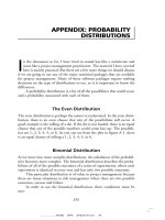
The Even Distribution
The even distribution is perhaps the easiest to understand. In the even distri-
bution, there is an even chance that any of the possibilities will occur. A
good example is the rolling of a die. If the die is not loaded, there is an equal
chance that any of the possible numbers could come face up. The possibili-
ties are 1, 2, 3, 4, 5, or 6. As you can see from the plot in figure A-1, there
is an equal chance of rolling a 1, 2, 3, 4, 5, or 6.
Binomial Distribution
As we move into more complex distributions, the calculation of the probabil-
ities becomes more complex. The binomial distribution describes the proba-
bilities of all of the possible outcomes of a series of experiments, where each
experiment is identical in every way and has only two possible outcomes.
This particular distribution is of value in project management because
there are many situations in risk management where there are two possible
outcomes, success and failure.
In order to use the binomial distribution, three conditions must be
met:
375
.......................... 9618$$ APPX 09-06-02 15:01:34 PS

376 Appendix: Probability Distributions
Figure A-1. Even distribution plot.
Probability
Possibilities
234561
1/3
1/4
1/6
1/12
1. Each event must have only two possible outcomes.
2. Each event must be statistically independent of the others. Statistical
independence means that the occurrence of one event does not have
an effect on the probability of any other event.
3. The probability of the outcome of any event must be the same from
event to event.
In the binomial distribution it is possible to calculate the value of the
probability directly. As the complexity of the distributions becomes more
and more complex, the formulas for making this calculation are too complex
to be done without the use of a computer.
P(x) ס [n! / (nמx)! x!] Π
x
(1מΠ)
nמx
Where: x is the number of occurrences of a particular outcome; P(x) is
the probability that x will occur; n is the number of events that will mea-
sured. Π is the probability of the outcome occurring in one event. ! stands
for factorial. Factorial means multiplying the number by successively smaller
integers until 1 is reached. 5! is 5 ן 4 ן 3 ן 2 ן 1 ס 120.
For example, suppose a coin is flipped three times. The probability of
getting a head on any flip is .5. What are the probabilities of getting two

heads in the five tries?
.......................... 9618$$ APPX 09-06-02 15:01:35 PS
377Appendix: Probability Distributions
The probability of two heads is:
P(2) ס [3! / (3מ1)! 3!] .5
2
(1מ.5)
1
P(2) ס (6 / 2) ן 0.25 ן 0.5 ס 0.375
Poisson Distribution
The Poisson distribution is used to describe the probabilities of independent
events spaced over time or some other parameter. This distribution is useful
in projects involving queues on lines and the number of occurrences of an
event over a time period.
Some rules to the Poisson distribution are:
1. Each occurrence must be statistically independent of the others.
2. There must be an expected number of events over a period of time.
3. The probability of more than one occurrence happening at the same
time is very small.
The Normal Distribution
From the illustration in figure A-2, it can be seen that the normal distribu-
tion curve is bell shaped, with a high point in the middle and an ever-
decreasing slope toward horizontal at the ends.
One of the important things about the normal distribution is that the
formula for calculating it depends on only two factors, the mean value and
the standard deviation. The mean value locates the middle of the curve, or
the peak. The standard deviation shows whether the curve is clustered tightly
around the midpoint or whether it is loosely clustered (figure A-3).
It has been found that most physical occurrences will fit a normal curve
or something close to it. This is true of many of the things that we would

like to approximate in project management. The probability distribution of
cost and schedule estimates fits this kind of distribution. In the area of sched-
uling, the PERT method is employed to more closely predict the completion
time for a project. In cost estimating, the normal distribution is used to
predict the range of values that has a given probability of occurring if that
project is actually done.
In PERT and cost estimating, we want a 95 percent probability of
.......................... 9618$$ APPX 09-06-02 15:01:36 PS
378 Appendix: Probability Distributions
Figure A-2. Normal distribution curve.
E؎2S, Probability is 95.5%
E؎3S, Probability is 99.7%
E
3S
2S
1S
E؎1S, Probability is 68.3%
Figure A-3. Standard deviation: A measurement of the
dispersion of the data.
Standard deviation=17
Standard deviation=5
Mean=22
Mean=22
being correct in our estimate. As in all probability distribution curves, the
area under the curve between the two points we are interested in compared
to the total area under the entire curve is the probability that the actual event
will be between the two values. This means that we can use the normal
distribution to determine the probability that the true value of our project
will be between two estimated values.
For convenience, multiples of the standard deviation are used to mark

off these ranges in values. The mean value of a project cost, for example, plus
or minus one (ע 1) standard deviation is 68.3%, ע2 standard deviations is
.......................... 9618$$ APPX 09-06-02 15:01:37 PS
379Appendix: Probability Distributions
95.5%, and ע3 standard deviations is 99.7%. These are values that are used
for convenience. Any range of values within the limits of the distribution
could be similarly calculated.
In the area of statistical quality control, the term ‘‘plus or minus 3
standard deviations’’ and the term ‘‘3 sigma’’ are frequently heard. Sigma is
the Greek letter usually used to represent standard deviation. In statistical
quality control, it is usual to want the accuracy of the inspection process to
have a 99.7% probability of being correct. That is a 99.7% chance that the
lot of parts that is inspected and deemed to be acceptable is really acceptable
and a 99.7% chance that a lot of parts that is said to be unacceptable is really
unacceptable. More is said about statistical quality control in chapter 6.
All normal curves have the same percentage of total area between the
same multiples of the standard deviation. Suppose point ‘‘a’’ is
1
/
2
standard
deviation above the mean value. Suppose another point called ‘‘b’’ is 2 stan-
dard deviations above the mean. The area or probability of the actual value
being between these two values is 28.57%.
Now suppose the mean value is 100, and the standard deviation is 10.
Point ‘‘a’’ would be 105, and point ‘‘b’’ would be 120. The probability of
the actual cost being between 105 and 120 is 28.57%.
If the standard deviation is 5 and the mean is 50, point ‘‘a’’ would be
52.5 and point ‘‘b’’ would be 60. The probability of the actual cost being
between 55 and 60 is 28.57%.

Most statistical computer programs make these calculations directly. In
fact most inexpensive calculators that have only the most basic statistical
functions perform these calculations.
In the appendix of most statistics books you will find Z tables. These
tables are used to find the probability or the area under the normal distribu-
tion curve for any point on the horizontal axes and the mean value. To use
the tables, standardize the values desired by dividing them by the standard
deviation.
In the previous example, the standard deviation was 10, the mean value
was 100, and the desired probability was between ‘‘a’’ at 105 and ‘‘b’’ at
120. To use the table we must standardize the values:
Z ס (x מ mean value) / standard deviation
Z for the ‘‘a’’ value ס 5/10ס .5
Z for the ‘‘a’’ value ס 20 / 10 ס 2.0
From this we can find the probability in the Z table for .5 and the
value for 2.0. Both of these values are on the same side of the mean, so we
.......................... 9618$$ APPX 09-06-02 15:01:39 PS