Socioeconomic environment and cancer incidence: A French population-based study in Normandy

Bryere et al. BMC Cancer 2014, 14:87
/>
RESEARCH ARTICLE

Open Access

Socioeconomic environment and cancer incidence:
a French population-based study in Normandy
Josephine Bryere1*, Olivier Dejardin1,2,6, Veronique Bouvier1,2,6, Marc Colonna3, Anne-Valérie Guizard1,4,6,
Xavier Troussard1,2,6, Carole Pornet1,2, Françoise Galateau-Salle1,2,6, Simona Bara1,5,6, Ludivine Launay1,
Lydia Guittet1,2 and Guy Launoy1,2,6

Abstract
Background: The struggle against social inequalities is a priority for many international organizations. The objective
of the study was to quantify the cancer burden related to social deprivation by identifying the cancer sites linked to
socioeconomic status and measuring the proportion of cases associated with social deprivation.
Methods: The study population comprised 68 967 cases of cancer diagnosed between 1997 and 2009 in
Normandy and collected by the local registries. The social environment was assessed at an aggregated level
using the European Deprivation Index (EDI). The association between incidence and socioeconomic status was
assessed by a Bayesian Poisson model and the excess of cases was calculated with the Population Attributable
Fraction (PAF).
Results: For lung, lips-mouth-pharynx and unknown primary sites, a higher incidence in deprived was observed
for both sexes. The same trend was observed in males for bladder, liver, esophagus, larynx, central nervous
system and gall-bladder and in females for cervix uteri. The largest part of the incidence associated with deprivation
was found for cancer of gall-bladder (30.1%), lips-mouth-pharynx (26.0%), larynx (23.2%) and esophagus (19.6%) in males
and for unknown primary sites (18.0%) and lips-mouth-pharynx (12.7%) in females. For prostate cancer and melanoma
in males, the sites where incidence increased with affluence, the part associated with affluence was respectively 9.6%
and 14.0%.
Conclusions: Beyond identifying cancer sites the most associated with social deprivation, this kind of study points to
health care policies that could be undertaken to reduce social inequalities.
Keywords: Cancer incidence, Socioeconomic inequalities, Registries, Population attributable fraction

Background
Cancer is one of the leading causes of mortality worldwide
and the second in the developed countries. It is thought to
be responsible for around 13% of the total number of
deaths, approximately 7.6 million persons dying from cancer in 2008. While cancer survival continues to improve
essentially thanks to progress in treating patients and to
screening, the observations concerning incidence are
much less encouraging. Social deprivation can be singled
out as responsible for part of this cancer incidence and the

* Correspondence:
1
U1086 INSERM Cancers & Preventions, Avenue du Général Harris, Caen
14076, France
Full list of author information is available at the end of the article

struggle against social inequalities in cancer constitutes a
priority for international organizations [1].
Public action to reduce this gradient must rely in part
on the proper assessment of the burden of cancer associated with social environment and on the knowledge of
the mechanisms underlying such inequalities.
Studies of this type have initially focused on mortality
data [2,3]. But it is important to differentiate between social disparities in incidence of cancer and social disparities
in survival as it was the case in the literature of the recent
years. The relationship between cancer incidence and socioeconomic status is dynamic and needs to be continuously monitored.
The mechanisms by which the social environment influences the risk of cancer are many and varied. None of

© 2014 Bryere et al.; licensee BioMed Central Ltd. This is an Open Access article distributed under the terms of the Creative
Commons Attribution License ( which permits unrestricted use, distribution, and

reproduction in any medium, provided the original work is properly credited. The Creative Commons Public Domain
Dedication waiver ( applies to the data made available in this article,
unless otherwise stated.


Bryere et al. BMC Cancer 2014, 14:87
/>
these mechanisms are exclusive and all interact. Based on
the work of previous authors, these mechanisms are organized in behavioral models focusing on individual determinants [4,5] (alcohol, tobacco, diet, physical exercise,
practice prevention, etc.), or contextual models focusing
on complexity determinants [6,7] (occupational exposure,
general exposure, access to health system, etc.). This complexity suggests that a proper evaluation of the social
environment should not be limited to any particular indicator such as financial resources, education or profession,
but should appreciate the social environment in its entire
individual and collective dimension. Geographical approaches are thus particularly relevant for studying the
link between social environment and cancer incidence.
Moreover, from a public health point of view, the measure
of the human cost of these inequalities at an aggregated
level is particularly relevant for potential further actions.
The objective of the study was to quantify the part of
the cancer burden related to social deprivation. We firstly
identified the cancer sites linked to the socioeconomic status of the living area and secondly measured for each one
the proportion of cases of cancer associated with social
deprivation.

Methods
Study population

The population comprised all cases of cancer diagnosed in
Calvados and Manche, two French departements in BasseNormandie, from 1997 to 2009 and recorded in the five

local registries: Calvados cancer registry, digestive Calvados
registry, Manche cancer registry, Malignant hematological
Basse-Normandie registry and Multicentral mesothelioma
registry. The whole population comprised 68 967 cases divided into 29 cancer sites (Table 1). According from INSEE
(Institut National de la Statistique et des Etudes Economiques), the population of Calvados and Manche is composed
of 48% of men and 52% of women which is equivalent to
the national distribution. The population is slightly older
than the national average. In Calvados and Manche, 47% of
individuals are under 40 years compared to 50% nationally,
and 26% are over 60 years compared to 23% nationally.
The economy is also less efficient with a GDP of 2.1%; it
stands at 3.1% nationally.
Variables

The clinical characteristics of the tumors were collected
by the registries in a standardized way ensuring the completeness and good quality of the data. The site, morphology, age, gender and diagnosis date were known for
every patient.
For all cases of cancer diagnosed, place of residence
was geolocalized with a Geographic Information System
(GIS) running on MAPINFO 10.0 and allocated to an
IRIS (Ilots Regroupes pour l'Information Statistique), a

Page 2 of 10

geographical area defined by INSEE [8]. It is the smallest
geographical unit for which census data are known, a factor essential for this kind of study [9]. There are 1496 IRIS
in the two departments. The smallest IRIS is composed of
10 inhabitants, the biggest is composed of 4811 inhabitants
and the mean is 755. The database provided the number of
cancer cases diagnosed in an IRIS for the whole period.

The reference population came from the INSEE social
census 1999 and 2006. It is given for each IRIS, each sex
and each age group: [0–14], [15–29], [30–44], [45–59],
[60–74], [75 and more]. The population was linearly extrapolated for the whole period 1997–2009. Knowing the
population sizes for an IRIS, an age group and a gender
for the years 1999 and 2006, supposing that an increase or
a decrease of the sizes were constant, we extrapolated the
population sizes for the years 1997, 1998, 2000, 2001,
2002, 2003, 2004, 2005, 2007, 2008, 2009.
The recently published French EDI (European Deprivation
Index) was used to attribute a social deprivation score
to the IRIS [10]. The methodology used an individual
deprivation indicator from the conceptual definition of
deprivation and selected ecological census variables that
are the most closely related to the individual deprivation
indicator in the European Union Statistics on Income and
Living Conditions (EU-SILC). This was available as a continuous variable, increasing from - 5.33 to 20.52. Depending on the modelling performed, the continuous version
of the EDI variable or a categorical version (quintiles calculated at the French level) was used.
Statistical analysis

A Bayesian approach was used rather than the classical
Poisson regression because it allows the integration of
extra-Poisson variability if it exists in the data. The differences in population sizes between IRIS, called unstructured spatial heterogeneity, may have introduced
variations and this methodology permits the distinction
between random fluctuations and true variations in incidence rates. Moreover, neighboring areas may not be independent and have similar incidence rates and this
phenomenon, called spatial autocorrelation, is also integrated with the Bayesian approach [11,12] performed
using WinBUGS version 1.4 [13]. It is written as follows:
logðyi Þ ¼ logðE i Þ þ α þ β EDI i þ V i þ U i
where yi and Ei are the
Xobserved and expected number of

cases in area i. E i ¼
t j;k P j;k where tj,k is the global incij;k

dence rate for the age group j and sex k and Pj,k is the
population size for the IRIS i, age group j and sex k. α is
the intercept, representing the global relative risk, β the
coefficient associated with the variable EDI, Ui is the structured variation (spatially structured heterogeneity) and Vi


Bryere et al. BMC Cancer 2014, 14:87
/>
Page 3 of 10

Table 1 Site definitions and frequencies in Normandy between 1997 and 2009
Site

ICD-O-3

Frequencies

Topographya

Morphologya

Men

Prostate

C61

All

11611

Breast

C50

All

Lung

C33, C34

All

6095

Women

Total
11611

10893

10893

1324

7419

Colon-rectum

C18, C19, C20, C21

All

3983

3206

7189

Lips-mouth-pharynx

C0, C10, C11,

All

3153

579

3732

2452

590

3042

Bladder

C12, C13, C14

All

C67

All

Kidney

C64, C65, C66, C68

All

1334

737

2071

Non-Hodgkin

All

95903-95963 or

1071

945

2016

lymphoma

96703-97193 or
97273-97293 or
98323-98343

Stomach

C16

All

1186

691

1877

Melanoma

C44

87203-87803

725

1063

1788

Unknown primary sites

C76, C809,

All

925

654

1579

Central nervous system

C70, C71, C72

≤ 91103 or ≤91800

719

Corpus uteri

C54

All

Pancreas

C25

All

Liver

C22

All

Esophagus

C15

All

Ovary

C56, C570, C571,

All excluding

C572, C573, C576

801

1520

1449

1449

786

660

1446

1148

238

1386

1138

208

1346

1247

1247

646

543

1189

258

884

1142

{84423; 84513;
84613; 84623;
84723; 84733}

Myeloma

All

Thyroid

C73

97313-97343 or
97603-97643
All

Larynx

C32

All

867

86

953

Lymphocytic leukemia

All

98233

508

409

917

Cervix uteri

C53

All

Leukemia

All

98013-98203 or

764

764

393

356

749

185

254

439

155

364

98263-98273 or
98353-98613 or
98663-98743 or
98913-99203 or
99483
Gall bladder and extrahepatic bilary tract

C23, C24

All

Testis

C62

All

400

Hodgkin’s lymphoma

All

96503-96673

209

400

Mesothelioma

C384

All

190

60

250

Small intestine

C17

All

98

91

197

All cancers

C00 to C80

All

40080

28887

68967

a

Hematological codes are always excluded from solid tumor sites and included in the relevant hematological site.

Bryere et al. BMC Cancer 2014, 14:87
/>
is the unstructured variation (non spatially structured heterogeneity). The EDI coefficient was estimated with its
95% credible intervals (CIs) for each cancer site. A positive
EDI parameter means an over-incidence in deprived areas
and a negative EDI parameter means an over-incidence in
affluent areas. We calculated exp (β) for significant sites
because it reflects the excess risk related to EDI. Living in
an IRIS with a highest deprivation score of one over another, increases the risk of developing a cancer of exp (β).
To know whether spatial autocorrelation and spatial
heterogeneity were actually in the data, we first performed a Moran test [14] for autocorrelation and a
Potthoff-Wintinghill test [15] for heterogeneity. They
were performed with packages spdep and DCluster
from R version 2.15.0, p-values of the tests being indicated in tables. If both tests were significant we performed a BYM (Besag, York and Mollié) model
integrating the two components, if just the Moran test
was significant we performed a CAR (Conditional Auto
Regressive) model integrating the spatially structured
heterogeneity, if just the Potthoff-Wintinghill test was
significant we performed a model with the nonspatially structured heterogeneity and if both tests
were non-significant, meaning that there was no variability of incidence in the data, the integration of EDI
was not included in the analysis.
The final step was to assess for each cancer site the
Population Attributable Fraction (PAF) [16,17]. It can be
defined [16] as the proportional reduction in average
disease risk over a specified time interval that would be
achieved by eliminating the exposure of interest from
the population. To do so, the national quintile version of
the deprivation index EDI was used and included in the
model. The quintiles were named Q1 to Q5, Q1 being the

quintile of the least deprived group and Q5 the quintile
of the most deprived one. A relative risk was determined
for each social deprivation level and was called RR1 to
RR5. The relative risks were calculated using the exact
same model as above, except that the categorical version
of the EDI (by quintile) was introduced into the model.
If a significant and a positive beta coefficient were observed, then Q1 was considered as the reference category. If a significant and a negative beta coefficient
were observed, then Q5 was considered as the reference
category. The relative risk of the reference category was
set to 1. The associated proportion of risk was defined
as:
PAF ¼ 1− X

1

p RRi
i¼1::5 i

Pi is the proportion of the population at the national
quintile i.

Page 4 of 10

Results
For the whole study period, 68 967 cases of cancer were
recorded in Calvados and Manche, 40 080 men and 28
887 women.
The most frequent sites in decreasing order were prostate, breast, lung, colon-rectum and lips-mouth-pharynx
(Table 1).
Concerning the continuous deprivation index EDI, the

minimum was −3.77 for the most affluent IRIS and the
maximum was 8.98 for the most deprived IRIS, the median being −0.45. Quintiles being defined at a national
level, 20% of the population was situated at the first
quintile, 22% at the second, 23% at the third, 23% at the
fourth and 12% at the fifth.
Tables 2 and 3 present the results of modelling using
the continuous version of EDI.
The Potthoff-Whittinghill test and the Moran test
were significant for a majority of sites.
The link between incidence and social deprivation was
not significant for a majority of cancer sites in both genders, was positive for 9 sites in males and 4 sites in females
and was negative for two in males and none in females.
For lung, lips-mouth-pharynx and unknown primary sites,
the link was positive in both genders. We obtained similar
betas for both genders but the sites concerned were more
frequent in males so the impact in terms of number of
cases was greater in males. The link was positive in males
only for bladder, liver, esophagus, larynx, central nervous
system and gall-bladder and in females only for cervix
uteri. The highest relative risks concerned lips-mouthpharynx in both genders, larynx and gall-bladder in males
and cervix uteri in females.
Tables 4 and 5 present the relative risks calculated
using the quintile version of EDI and the results of the
calculation of the PAF.
Using the calculation of PAF, the greatest part of the
incidence associated with deprivation was found for lipsmouth-pharynx cancer, esophageal cancer, laryngeal cancer and gall-bladder in males, respectively 26.0%, 19.6%,
23.2% and 30.1%. In females, the greatest part of the incidence associated with deprivation was found for unknown primary sites (18.0%) and lips-mouth-pharynx
(12.7%). For prostate cancer and melanoma in males, the
sites where incidence increased with affluence, the part associated with affluence was respectively 9.6% and 14.0%.
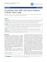
The excess cases due to social deprivation are represented

in Figures 1 and 2. The highest number of cases attributable to social deprivation concerned lips-mouth-pharynx
cancer in males (n = 820) (Figure 1) and unknown primary
sites (n = 120) (Figure 2) in females and for prostate cancer, 1115 cases can be considered as excess cases due to
affluence and for melanoma in males, 90 cases can be considered as excess cases due to affluence. By adding excess
cases associated with deprivation, we find 2287 excess


Bryere et al. BMC Cancer 2014, 14:87
/>
Page 5 of 10

Table 2 Influence of socioeconomic deprivation of living area on cancer incidence in men in Normandy between 1997
and 2009
Site
Prostate

Moran test

PW test

Estimationa

p-value

p-value

EDI coefficient

0.33

< 0.05

−0.023

CIb (95%)

Exp (β)

[−0.043; -0.010]

0.98
1.09

Lung

< 0.025

< 0.05

0.087

[0.065; 0.108]

Colon-rectum

< 0.025

< 0.05

0.025

[−0.001; 0.050]

Lips-mouth-pharynx

< 0.025

< 0.05

0.149

[0.122; 0.176]

1.16

Bladder

< 0.025

< 0.05

0.033

[0.001; 0.064]

1.03

Kidney

<0.025

< 0.05

0.033

[−0.003; 0.069]

Stomach

< 0.025

< 0.05

0.001

[−0.047; 0.047]

Liver

< 0.025

< 0.05

0.076

[0.039; 0.114]

1.08

Esophagus

< 0.025

< 0.05

0.086

[0.043; 0.131]

1.09

Non-Hodgkin lymphoma

0.04

< 0.05

−0.006

[−0.047; 0.035]

Unknown primary sites

0.11

< 0.05

0.060

[0.019; 0.101]

1.06

Larynx

< 0.025

< 0.05

0.154

[0.114; 0.196]

1.17

Pancreas

0.65

< 0.05

0.019

[−0.029; 0.066]

Melanoma

0.86

< 0.05

−0.078

[−0.132; -0.026]

0.92

Central nervous system

< 0.025

< 0.05

0.056

[0.010; 0.101]

1.06

Myeloma

0.84

< 0.05

−0.024

[−0.080; 0.030]

Lymphocytic leukemia

0.98

< 0.05

−0.040

[−0.105; 0.023]

Testis

< 0.025

< 0.05

−0.029

[−0.094; 0.036]

Leukemia

0.43

< 0.05

−0.013

[−0.080; 0.052]

Thyroid

0.09

< 0.05

0.020

[−0.057; 0.095]

Hodgkin’s lymphoma

0.16

< 0.05

−0.085

[−0.180; 0.005]

Gall-bladder and

< 0.025

< 0.05

0.141

[0.058; 0.221]

Mesothelioma

< 0.025

< 0.05

0.057

[−0.172; 0.052]

Small intestine

0.69

< 0.05

0.009

[−0.127; 0.135]

1.15

Extrahepatic bilary tract

a

Positive for an over-incidence in deprived areas, negative otherwise.
Significant CIs are in bold type.

b

cases in men (5.7% of the total number of cancers in men)
and 353 in females (1.2% of the total number of cancer in
females).

Discussion
This study provides evidence of social disparities in the
incidence of cancers. Most of these disparities consist in
an over-incidence for the most deprived, especially for
lips-mouth-pharynx, lung, unknown primary sites, bladder and larynx cancers. Both genders are concerned, but
the impact is greater in men, considering the huge frequency of these cancer sites for them. These inequalities
in incidence are all the more serious and the cancer burden is all the greater in that the cancer sites concerned
are those associated with very low survival. For the
period 1997–2009, analysis with the PAF showed that
the social gradient generated 2287 (5.7%) excess cases in
men and 353 (1.2%) in females. By analyzing site by site,

the social gradient generated up to 30.1% (gall-bladder)
and 18.0% (unknown primary sites) extra cases in men
and women respectively.
The sites identified as linked with socioeconomic
status are not surprising and consistent with previous papers. Thus, the highest incidence for lung, lips-mouthpharynx, esophagus, larynx, bladder and liver cancer in
low socioeconomic status can be explained by a higher
consumption of alcohol and tobacco in the most disadvantaged [5,18,19]. Similarly, the trend in over-incidence
of cervical cancer in deprived women can be explained
by sexual behaviors and/or lower participation in pap
smear screening [20]. The highest incidence of cancers
with unknown primary sites in males and females with
a low socioeconomic status can be explained by the fact
that the group of “unknown primary sites” mainly comprised subjects with metastatic cancers where the primary site could not be identified, a situation more

Bryere et al. BMC Cancer 2014, 14:87
/>
Page 6 of 10

Table 3 Influence of socioeconomic deprivation of living area on cancer incidence in females in Normandy between
1997 and 2009
Moran test

PW test

Estimationa

p-value

p-value

EDI coefficient

Breast

< 0.025

< 0.05

−0.016

[−0.032; 0.001]

Colon-rectum

< 0.025

< 0.05

−0.001

[−0.026; 0.026]

Corpus uteri

< 0.025

< 0.05

0.024

[−0.011; 0.059]

Site

CIb (95%)

Lung

< 0.025

< 0.05

0.075

[0.037; 0.113]

Ovary

0.69

< 0.05

−0.031

[−0.069; 0.006]

Melanoma

0.49

< 0.05

−0.028

[−0.068; 0.012]

Non-Hodgkin lymphoma

0.79

< 0.05

−0.004

[−0.046; 0.038]

Thyroid

< 0.025

< 0.05

0.002

[−0.043; 0.047]

Central nervous system

< 0.025

< 0.05

0.024

[−0.044; 0.051]

Cervix uteri

< 0.025

< 0.05

0.094

[0.052; 0.136]

Kidney

< 0.025

< 0.05

0.021

[−0.026; 0.068]

Stomach

< 0.025

< 0.05

0.007

[−0.052; 0.067]

Pancreas

0.05

< 0.05

0.045

[−0.004; 0.091]

Unknown primary site

0.56

< 0.05

0.065

[0.015; 0.113]

Bladder

< 0.025

< 0.05

0.033

[−0.023; 0.086]

Lips-mouth-pharynx

< 0.025

< 0.05

0.103

[0.054; 0.150]

Myeloma

0.35

< 0.05

−0.038

[−0.096; 0.020]

Lymphocytic leukemia

< 0.025

< 0.05

0.041

[0.024; 0.104]

Leukemia

0.04

< 0.05

−0.036

[−0.107; 0.034]

Gall-Bladder and

0.93

< 0.05

−0.014

[−0.097; 0.068]

Exp (β)

1.08

1.10

1.08

1.11

Extrahepatic bilary tract
Liver

< 0.025

< 0.05

0.078

[−0.002; 0.154]

Esophagus

0.40

< 0.05

0.068

[−0.017; 0.151]

Hodgkin’s lymphoma

0.33

0.11

Small intestine

0.88

0.14

Larynx

< 0.025

0.06

0.110

[−0.005; 0.217]

Mesothelioma

< 0.025

0.05

0.040

[−0.144; 0.205]

a

Positive for an over-incidence in deprived areas, negative otherwise.
Significant CIs are in bold type.

b

frequent in people with a low socioeconomic status
[21]. Results in the literature concerning the relation
between incidence of central nervous system cancer socioeconomic status are contradictory. The etiology of
cerebral tumors remains unclear [22,23]. The results
concerning gall-bladder are consistent with previous
papers. People with a low socioeconomic status may
have a diet and a feeding behavior which contribute to a

development of the disease [24]. The trend in overincidence of prostate cancer may come from the higher
participation of high socioeconomic classes in screening
activities and since PSA screening is associated with over
diagnosis [25]. The higher participation of high socioeconomic classes in screening activities can also explain the
higher incidence for affluent patients for melanoma in
males and this higher incidence can also be explained by

holidays abroad and exposure to natural UV [17,26]. Conversely, the absence of a social gradient in the incidence of
breast seems surprising, since it is targeted by screening
associated with social inequalities in participation, and
because well-established risk factors such as late age at
first birth or hormone replacement are more prevalent
in high socioeconomic groups [6]. The spatial nature of
the data and its specificities (spatial autocorrelation and
non spatially structured heterogeneity) was accounted in
our modelling thanks to the Bayesian approach ensuring a
good consistency of the statistical analysis. Such a methodology was not integrated in previous studies treating cancer incidence and social disparities, preferring a classical
Poisson regression, and thus risking to underestimate the
standard error and to wrongly conclude at a significant effect of deprivation on cancer incidence [27].


Bryere et al. BMC Cancer 2014, 14:87
/>
Page 7 of 10

Table 4 Analysis using the quintile version of EDI and
Population Attributable Fraction in males between 1997
and 2009
RR

CI

PAFa (%)

Quintile 1

1.19

[1.09; 1.29]

9.6

Quintile 2

1.13

[1.04; 1.22]

Quintile 3

1.04

Quintile 4

1.15

Site
Prostate

Lung

Lips-mouth-pharynx

Bladder

Liver

Esophagus

Unknown primary sites

Larynx

Table 4 Analysis using the quintile version of EDI and
Population Attributable Fraction in males between 1997
and 2009 (Continued)
Quintile 1

1.37

[1.07; 1.77]

Quintile 2

1.16

[0.89; 1.49]

Quintile 3

1.06

[0.82; 1.37]

[0.96; 1.12]

Quintile 4

1.18

[0.92; 1.50]

[1.06; 1.24]

Quintile 5

1

Quintile 5

1

Quintile 1

1

Quintile 2

1.07

Quintile 3

0.99

Quintile 4

1.18

[1.06; 1.31]

Quintile 5

1.44

[1.29; 1.61]

Quintile 1

1

Quintile 2

1.23

[1.06; 1.43]

Quintile 3

1.20

Quintile 4

Melanoma

Central nervous system

Quintile 1

1

Quintile 2

1.05

[0.81; 1.35]

[0.97; 1.19]

Quintile 3

1.16

[0.91; 1.47]

[0.88; 1.10]

Quintile 4

1.15

[0.90; 1.44]
[0.93; 1.54]

9.9

9.4

Quintile 5

1.19

Quintile 1

1

Quintile 2

1.59

[0.94; 2.80]

Quintile 3

1.32

[0.77; 2.27]

[1.03; 1.39]

Quintile 4

1.31

[0.90; 2.60]

1.54

[1.34; 1.78]

Quintile 5

1.88

[1.11; 3.24]

Quintile 5

2.05

[1.77; 2.05]

Quintile 1

1

Quintile 2

1.10

[0.95; 1.27]

Quintile 3

0.93

[0.80; 1.09]

Quintile 4

1.51

[0.99; 1.34]

Quintile 5

1.19

[1.01; 1.40]

Quintile 1

1

Quintile 2

1.04

[0.85; 1.27]

Site

Quintile 3

0.93

[0.75; 1.14]

Lung

Quintile 4

1.14

[0.94; 1.38]
[1.15; 1.71]

Gall-bladder
26.0

30.1

a

6.0

PAF calculated with quintile 1 as reference except for prostate cancer
and melanoma.

6.9

Table 5 Analysis using the quintile version of EDI and
Population Attributable Fraction in females between
1997 and 2009
RR

CI

Quintile 1

1

Quintile 2

1.09

[0.88; 1.35]

Quintile 3

1.12

[0.84; 1.29]

Quintile 4

1.10

[0.89; 1.35]

Quintile 5

1.37

[1.11; 1.71]

Quintile 1

1

Quintile 5

1.40
1

Quintile 2

1.30

[1.05; 1.63]

Quintile 3

1.17

[0.95; 1.47]

Quintile 4

1.24

[1.01; 1.54]

Quintile 2

0.88

[0.67; 1.15]

Quintile 5

1.67

[1.34; 2.11]

Quintile 3

1.05

[0.81; 1.35]

Quintile 4

1.09

[0.86; 1.39]

Quintile 5

1.40

[1.10; 1.80]

19.6

Quintile 1

1
0.99

[0.79; 1.26]

Quintile 3

1.12

[0.89; 1.41]

Quintile 4

1.18

[0.95; 1.47]
[1.03; 1.65]

Cervix uteri

9.7

Quintile 5

1.13

Quintile 1

1

Quintile 2

1.05

[0.81; 1.35]

Quintile 3

1.24

[0.98; 1.58]

Quintile 4

1.54

Quintile 5

1.91

Unknown primary sites

23.2

5.2

Quintile 1

1

Quintile 2

1.21

[0.89; 1.65]

18.0

Quintile 3

1.15

[0.84; 1.54]

Quintile 4

1.43

[1.08; 1.91]
[0.95; 1.74]

Quintile 5

1.29

Quintile 1

1

[1.22; 1.95]

Quintile 2

0.98

[0.72; 1.35]

[1.49; 2.45]

Quintile 3

1.08

[0.78; 1.47]

Quintile 4

1.29

[0.96; 1.72]

Quintile 5

1.52

[1.11; 2.05]

Lips-mouth-pharynx

a

PAF calculated with quintile 1 as reference.

PAFa (%)
9.0

Quintile 1

Quintile 2

14.0

12.7


Bryere et al. BMC Cancer 2014, 14:87
/>
Page 8 of 10

7000

6000
603

Number of cases

5000

4000

3000
820

147

2000

223

79

90

1000

201

68
56

0

Expected

Excess

Figure 1 Proportion of excess cases associated with social deprivation in men.

Our study has several limits. By using the PAF and in
absence of individual data, we sought to quantify social inequalities in incidence of cancer, rather than understand
the underlying mechanisms. Using a neighborhood-based
index instead of a set of individual indicators has the advantage of incorporating both individual and collective determinants that jointly mediate the social environment,

but this inevitably introduces an ecological bias for appropriate measurement of individual socioeconomic status.
Moreover, it considerably limits the search for causative factors explaining the links between social environment and
occurrence of cancer, individual measures of socioeconomic
status and behavioral risk factors being the best means to
explore in more depth the mechanisms responsible for the

7000

6000

Number of cases

5000

4000

3000

2000
119
40

1000

0

Lung

Cervix
Expected

74

Lips-Mouth-Pharynx
Excess

Figure 2 Proportion of excess cases associated with social deprivation in women.

120

unknown primary site


Bryere et al. BMC Cancer 2014, 14:87
/>
influence of social environment on cancer risk. In addition,
the social environment was measured only at the time of
diagnosis, using the current address of patients but ignoring
their history of mobility, which could be geographical and
across social classes. Furthermore, we focused on the consequences of previous social inequalities owing to the delay
between exposure and diagnosis. Despite the large number

of cases analyzed from cancer registries that have a high
level of case ascertainment, consistency and representativeness, a lack of power cannot be excluded for the less frequent cancer sites.
Extrapolation of the PAFs needs further investigations
in order to ascertain their variability due to gradient in
relative risks, or to distribution across social quintiles.
Errors in interpretation can appear, as highlighted in the
article by Rockhill, et al. [16] with the use of the PAF.
Firstly, Rockhill et al. point out many errors possible
when analyzing multiple risk factors which is not the
case of our study. The second point is the overuse of the
word “explain” in the interpretation of the PAF. Rather
than explain, it measures the extent of the phenomenon
of deprivation on cancer incidence. The PAF should be
considered as the population resultant of the overall excess of cases in deprived compared with privileged
people. The socioeconomic environment is not a causal
factor of cancer in the biological sense of the term.
However, since much of the proximal risk factor is more
prevalent in the deprived, the socioeconomic environment can be considered as the "cause of the cause", a
distal determinant, pathways from deprivation to health
including different types of mediators such as behavioral, community, social, educational, work-related, cultural and political factors [28]. Such quantification of
social disparities at a community level points to the
need to jointly take actions in a universal approach and
also in approaches targeting deprived people, rather
than global population actions only that fail to reduce
social gradients because they generally benefit the more
affluent. The PAF makes it possible to estimate the collective gain that could be obtained by public actions
aiming to reduce the social gradient of incidence by
measuring the extent of the population for which it is
necessary to lead effective cancer prevention.

Conclusions
This study proposes an estimation of the proportion of
cancers associated with social deprivation and show how
by decreasing socioeconomic variation in incidence with
policies aiming to reduce social inequalities, an important impact could be made on the burden of cancer.
Competing interests
The authors declare that they have no competing interests.

Page 9 of 10

Authors’ contribution
JB, OD and GL worked on the conception and design. OD, VB, AVG, XT, FGS,
SB, CP and LL participated in the acquisition of data. JB performed the
analysis and interpreted the data with OD, VB, MC, LG and GL. JB, OD, VB,
MC, CP, LG and GL revised the manuscript and all authors read and
approved the final manuscript.
Acknowledgments
We thank INSERM (Institut National de la Sante et de la Recherche Medicale)
and the Basse-Normandie regional government that have supported this
work.
Author details
1
U1086 INSERM Cancers & Preventions, Avenue du Général Harris, Caen
14076, France. 2CHU, Avenue de la Côte de Nacre, Caen 14000, France. 3Isere
cancer registry, CHU, Grenoble, France. 4CRLCC, Avenue du Général Harris,
Caen 14076, France. 5Public hospital, rue Trottebec, Cherbourg 50100, France.
6
Federation of cancer registries of Basse-Normandie, Caen, France.
Received: 18 November 2013 Accepted: 12 February 2014
Published: 13 February 2014

References
1. World Health Organization. www.who.int/topics/cancer/en/.
2. Mackenbach JP, Stirbu I, Roskam A: Socioeconomic inequalities in health
in 22 European countries. N Engl J Med 2008, 358:2468–81.
3. Menvielle G, Leclerc A, Chastang JF, Melchior M, Luce D: Changes in
socioeconomic inequalities in cancer mortality rates among French men
between 1968 and 1996. Am J Public Health 2007, 97:2082–7.
4. Faggiano F, Partanen T, Kogevinas M, Boffeta P: Socioeconomic difference
in cancer incidence and mortality. IARC Sci Publ 1997, 138:65–176.
5. Merletti F, Galassi C, Spadea T: The socioeconomic determinants of
cancer. Environ Health 2009, 10:S7.
6. Robert SA, Strombom I, Trentham-Dietz A, Hampton JM, McElroy JA,
NewComb PA, Remington PL: Socioeconomic risk factors for breast cancer.
Distinguishing individual- and community-level effects. Epidemiology 2004,
15:442–50.
7. Sanderson M, Coker AL, Perez A, Du XL, Peltz G, Fadden MK: A multilevel
analysis of socioeconomic status and prostate cancer risk. Ann Epidemiol
2006, 16:901–7.
8. Institut National de la Statistique et des Etudes Economiques (INSEE).
/>9. Woods LM, Rachet B, Coleman MP: Choice of geographic unit influences
socioeconomic inequalities in breast cancer survival. Br J Cancer 2005,
92:1279–1282.
10. Pornet C, Delpierre C, Dejardin O, Grosclaude P, Launay L, Guittet L, Lang T,
Launoy G: Construction of an adaptable European transnational
ecological deprivation index: the French version. J Epidemiol Community
Health 2012, 66:982–9.
11. Colonna M: Influence des paramètres a priori dans l’estimation
bayésienne de risques relatifs. Analyse spatiale du cancer de la vessie
dans l’agglomération grenobloise. Rev Epidemiol Sante Publique 2006,
54:529–42.

12. Pascutto C, Wakefield JC, Best NG, Richardson S, Bernardinelli L, Staines A,
Elliott P: Statistical issues in the analysis of disease mapping data.
Stat Med 2000, 19:2493–519.
13. Spiegelhalter DJ, Thomas A, Best N: Winbugs version 1.4 software and
user manual. Cambridge 2004.
14. Ancelet S: Exploiter l’approche hiérarchique bayésienne pour la
modélisation statistique des structures spatiales. Paris: PhD Thesis, AGRO
PARIS TECH, UMR518 Mathématiques et Informatique Appliqués; 2008.
15. Potthoff R, Whittinghill M: Testing for homogeneity: the binomial and
multinomial distributions. Biometrika 1966, 53:167–82.
16. Rockhill B, Newman B, Weinberg C: Use and misuse of population
attributable fractions. Am J Public Health 1998, 88:15–9.
17. Shack L, Jordan C, Thomson CS, Mak V, Moller H: Variation in incidence of
breast, lung and cervical cancer and malignant melanoma of skin by
socioeconomic group in England. BMC Cancer 2008, 8:271.
18. Dalton SO, Steding-Jessen M, Engholm G, Schuz J, Olsen JH: Social inequality
in incidence of and survival from lung cancer in a population-based study
in Denmark, 1994–2003. Eur J Cancer 2008, 44:2074–85.


Bryere et al. BMC Cancer 2014, 14:87
/>
Page 10 of 10

19. Shebl FM, Capo-Ramos DE, Graubard BI, Mc Glynn KA, Altekruse SF:
Socioeconomic status and hepatocellular carcinoma in the United States.
Cancer Epidemiol Biomarkers Prev 2012, 21:1330–5.
20. Singh GK, Miller BA, Hankey BF, Edwards BK: Persistent area socioeconomic
disparities in U.S. incidence of cervical cancer, mortality, stage, and
survival, 1975–2000. Cancer 2004, 101:1081–7.

21. Luke C, Koczwara B, Karapetis C, Pittman K, Price T, Kotasek D, Beckmann K,
Brown M, Roder D: Exploring the epidemiological characteristics of
cancers of unknown primary site in an Australian population:
implications for research and clinical care. Aust N Z J Public Health 2008,
32:383–9.
22. Spadea T, d’Errico A, Demeria M, Faggiano F, Pasian S, Zanetti R, Rosso S,
Vicari P, Costa G: Educational inequalities in cancer incidence in Turin,
Italy. Eur J Cancer Prev 2009, 18:169–78.
23. Mackillop W, Zhang-Salomons J, Boyd CJ, Groome PA: Associations
between community income and cancer incidence in Canada and the
United States. Cancer 2000, 89:901–12.
24. Ram KJ, Tewari M, Rai A, Sinha R, Mohapatra S, Shukla H: An objective
assessment of demography of gallbladder cancer. J Surg Oncol 2006,
93:610–4.
25. Welch HG, Albertsen PC: Prostate cancer diagnosis and treatment after
the introduction of prostate-specific antigen screening. J Natl Cancer Inst
2009, 101:1325–1329.
26. Eberle A, Luttmann S, Foraita R, Pohlabeln H: Socioeconomic inequalities
in cancer incidence and mortality – a spatial analysis in Bremen,
Germany. J Public Health 2010, 18:227–235.
27. Haining R, Law J, Griffith D: Modelling small area counts in the presence
of overdispersion and spatial autocorrelation. Comput Stat Data An 2009,
53:2923–37.
28. Jaarsveld C, Miles A, Wardle J: Pathways from deprivation to health
differed between individual and neighborhood-based indices. J Clin
Epidemiol 2007, 60:712–9.
doi:10.1186/1471-2407-14-87
Cite this article as: Bryere et al.: Socioeconomic environment and cancer
incidence: a French population-based study in Normandy. BMC Cancer
2014 14:87.

Submit your next manuscript to BioMed Central
and take full advantage of:
• Convenient online submission
• Thorough peer review
• No space constraints or color figure charges
• Immediate publication on acceptance
• Inclusion in PubMed, CAS, Scopus and Google Scholar
• Research which is freely available for redistribution
Submit your manuscript at
www.biomedcentral.com/submit