Bai giang math4
Bạn đang xem bản rút gọn của tài liệu. Xem và tải ngay bản đầy đủ của tài liệu tại đây (673.18 KB, 90 trang )
H ANOI U NIVERSITY OF S CIENCE AND T ECHNOLOGY
S CHOOL OF A PPLIED M ATHEMATICS AND I NFORMATICS
N GUYEN T HI T HU H UONG AND T RAN M INH T OAN
Lecture on
M ATH 4
M ULTIPLE I NTEGRAL , I NTEGRAL THAT DEPENDS ON A PARAMETER ,
L INE I NTEGRAL , S URFACE I NTEGRAL , F IELD T HEORY AND S ERIES
Summary, Examples, Exercises and Solutions
Ha Noi - 2008
C ONTENTS
Contents.
. . . . . . . . . . . . . . . . . . . . . . . . . . . . .
1
Chapter 1 . Multiple Integral . . . . . . . . . . . . . . . . . . . . . . . .
5
1
Double Integral . . . . . . . . . . . . . . . . . . . . . . . . . . . . . . . .
1.1
Calculation of a double integral in Cartesian coordinate system
1.2
Change of variables in double integrals, polar coordinate . . . .
1.3
Applications of double integrals . . . . . . . . . . . . . . . . . . .
1.4
Exercises . . . . . . . . . . . . . . . . . . . . . . . . . . . . . . . .
1.5
Solutions . . . . . . . . . . . . . . . . . . . . . . . . . . . . . . . .
2
Triple Integral . . . . . . . . . . . . . . . . . . . . . . . . . . . . . . . . .
2.1
Calculation of a triple integral in Cartesian coordinate system .
2.2
Change of variables in triple integrals . . . . . . . . . . . . . . .
2.3
Calculate the triple integrals in cylindrical coordinate . . . . .
2.4
Calculate the triple integrals in spherical coordinate . . . . . .
2.5
Exercises . . . . . . . . . . . . . . . . . . . . . . . . . . . . . . . .
2.6
Solutions . . . . . . . . . . . . . . . . . . . . . . . . . . . . . . . .
Chapter 2 . Integrals that depend on a parameter . . . . . . . . . . .
.
.
.
.
.
.
.
.
.
.
.
.
.
.
.
.
.
.
.
.
.
.
.
.
.
.
.
.
.
.
.
.
.
.
.
.
.
.
.
.
.
5
5
8
12
14
17
20
20
22
22
24
24
25
. 29
.
.
.
.
.
.
.
.
.
.
.
.
.
.
.
.
.
.
.
.
.
.
.
.
.
.
.
.
.
29
29
29
32
32
33
33
34
35
. 39
Line integral of the first kind . . . . . . . . . . . . . . . . . . . . . . . . . . .
39
1
The definite integrals that depend on a parameter . . .
1.1
Definition . . . . . . . . . . . . . . . . . . . . . . .
1.2
Properties . . . . . . . . . . . . . . . . . . . . . .
2
The generalized integarls that depend on a parameter .
2.1
The uniformly convergent integrals . . . . . . . .
2.2
Properties . . . . . . . . . . . . . . . . . . . . . .
2.3
Euler’s integrals . . . . . . . . . . . . . . . . . . .
3
Exercises . . . . . . . . . . . . . . . . . . . . . . . . . . .
4
Solutions . . . . . . . . . . . . . . . . . . . . . . . . . . .
Chapter 3 . Line integral . . . . . . . . . . . . . . . .
1
1
.
.
.
.
.
.
.
.
.
.
.
.
.
.
.
.
.
.
.
.
.
.
.
.
.
.
.
.
.
.
.
.
.
.
.
.
.
.
.
.
.
.
.
.
.
.
.
. .
.
.
.
.
.
.
.
.
.
.
. . .
. . .
. . .
. . .
. . .
. . .
. . .
. . .
. . .
. .
2
CONTENTS
1.1
Definition . . . . . . . . . . . . . . . . . . .
1.2
Calculation formulae . . . . . . . . . . . .
2
Line integral of the second kind . . . . . . . . . .
2.1
Definition . . . . . . . . . . . . . . . . . . .
2.2
Calculation formulae . . . . . . . . . . . .
2.3
Theorem of four equivalent propositions .
2.4
Area of a plane domain . . . . . . . . . . .
3
Exercises . . . . . . . . . . . . . . . . . . . . . . .
4
Solution . . . . . . . . . . . . . . . . . . . . . . . .
Chapter 4 . Surface integral . . . . . . . . . . . .
1
.
.
.
.
.
.
.
.
.
.
. . .
. . .
. . .
. . .
. . .
. . .
. . .
. . .
. . .
. .
.
.
.
.
.
.
.
.
.
.
.
.
.
.
.
.
.
.
.
.
.
.
.
.
.
.
.
.
.
.
.
.
.
.
.
.
.
.
.
.
.
.
.
.
.
.
.
. .
.
.
.
.
.
.
.
.
.
.
. . .
. . .
. . .
. . .
. . .
. . .
. . .
. . .
. . .
. .
.
.
.
.
.
.
.
.
.
.
.
.
.
.
.
.
.
.
.
.
.
.
.
.
.
.
.
.
.
39
39
41
41
41
45
46
46
49
. 53
Surface integral of the first kind .
1.1
Definition . . . . . . . . . . .
1.2
Calculation formulae . . . .
2
Surface integral of the second kind
2.1
Definition . . . . . . . . . . .
2.2
Calculation formulae . . . .
2.3
Stokes’ formula . . . . . . .
3
Exercises . . . . . . . . . . . . . . .
4
Solution . . . . . . . . . . . . . . . .
Chapter 5 . Field theory . . . . . . . .
. . .
. . .
. . .
. . .
. . .
. . .
. . .
. . .
. . .
. .
.
.
.
.
.
.
.
.
.
.
.
.
.
.
.
.
.
.
.
.
.
.
.
.
.
.
.
.
.
.
.
.
.
.
.
.
.
.
.
.
.
.
.
.
.
.
.
. .
.
.
.
.
.
.
.
.
.
.
. . .
. . .
. . .
. . .
. . .
. . .
. . .
. . .
. . .
. .
.
.
.
.
.
.
.
.
.
.
.
.
.
.
.
.
.
.
.
.
.
.
.
.
.
.
.
.
.
.
.
.
.
.
.
.
.
.
.
.
.
.
.
.
.
.
.
. .
.
.
.
.
.
.
.
.
.
.
. . .
. . .
. . .
. . .
. . .
. . .
. . .
. . .
. . .
. .
.
.
.
.
.
.
.
.
.
.
.
.
.
.
.
.
.
.
.
.
.
.
.
.
.
.
.
.
.
53
53
53
54
54
55
58
59
60
. 63
1
Scalar field
2
Vector field
3
Exercises .
4
Solution . .
Chapter 6 . Series
.
.
.
.
.
.
.
.
1
2
3
.
.
.
.
.
.
.
.
.
.
.
.
.
.
.
.
.
. .
.
.
.
.
.
. . .
. . .
. . .
. . .
. .
.
.
.
.
.
.
.
.
.
.
.
.
.
.
.
.
.
.
.
.
.
.
. .
.
.
.
.
.
. . .
. . .
. . .
. . .
. .
.
.
.
.
.
.
.
.
.
.
.
.
.
.
.
.
.
.
. .
.
.
.
.
.
. . .
. . .
. . .
. . .
. .
.
.
.
.
.
.
.
.
.
.
.
.
.
.
.
.
.
.
. .
.
.
.
.
.
. . .
. . .
. . .
. . .
. .
.
.
.
.
.
.
.
.
.
.
.
.
.
.
63
64
66
66
. 69
Number series . . . . . . . .
1.1
Definition . . . . . . .
1.2
Convergent criterion
1.3
Exercises . . . . . . .
1.4
Solution . . . . . . . .
Function series . . . . . . .
2.1
Function sequence .
2.2
Function series . . .
2.3
Power series . . . . .
2.4
Exercises . . . . . . .
2.5
Solution . . . . . . . .
Fourier series . . . . . . . .
.
.
.
.
.
.
.
.
.
.
.
.
.
.
.
.
.
.
.
.
.
.
.
.
.
.
.
.
.
.
.
.
.
.
.
.
.
.
.
.
.
.
.
.
.
.
.
.
.
.
.
.
.
.
.
.
.
.
.
.
.
.
.
.
.
.
.
.
.
.
.
.
.
.
.
.
.
.
.
.
.
.
.
.
.
.
.
.
.
.
.
.
.
.
.
.
.
.
.
.
.
.
.
.
.
.
.
.
.
.
.
.
.
.
.
.
.
.
.
.
.
.
.
.
.
.
.
.
.
.
.
.
.
.
.
.
.
.
.
.
.
.
.
.
.
.
.
.
.
.
.
.
.
.
.
.
.
.
.
.
.
.
.
.
.
.
.
.
.
.
.
.
.
.
.
.
.
.
.
.
.
.
.
.
.
.
.
.
.
.
.
.
.
.
.
.
.
.
.
.
.
.
.
.
.
.
.
.
.
.
.
.
.
.
.
.
.
.
.
.
.
.
.
.
.
.
.
.
69
69
70
74
75
78
78
78
80
82
83
85
.
.
.
.
.
.
.
.
.
.
.
.
.
.
.
.
.
.
.
.
.
.
.
.
.
.
.
.
.
.
.
.
.
.
.
.
.
.
.
.
.
.
.
.
.
.
.
.
.
.
.
.
.
.
.
.
.
.
.
.
.
.
.
.
.
.
.
.
.
.
.
.
.
.
.
.
.
.
.
.
.
.
.
.
.
.
.
.
.
.
.
.
.
.
.
.
.
.
.
.
.
.
.
.
.
.
.
.
CONTENTS
3.1
3.2
3.3
3
Decomposition theorem . . . . . . . . . . . . . . . . . . . . . . . . . . .
Exercises . . . . . . . . . . . . . . . . . . . . . . . . . . . . . . . . . . .
Solution . . . . . . . . . . . . . . . . . . . . . . . . . . . . . . . . . . . .
85
89
89
4
CONTENTS
CHAPTER
1
M ULTIPLE I NTEGRAL
§1. D OUBLE I NTEGRAL
1.1 Calculation of a double integral in Cartesian
coordinate system
Consider the integral
I=
f ( x, y)dxdy.
(1.1)
D
1. (The Corollary of Fubini’s theorem)
Suppose that D = [ a, b] × [c, d] and f : D → R is a continuous function on D. Then
I=
f ( x, y)dy =
dx
a
b
d
d
b
c
c
f ( x, y)dx
dy
a
a ≤ x ≤ b
2. If D is described as follows: D =
,
ϕ( x ) ≤ y ≤ ψ( x )
where y = ϕ( x ), y = ψ( x) are continuous and have continuous derivatives on [ a, b]
ψ( x )
b
then I =
a
ϕ( x )
f ( x, y)dy dx or
ψ( x )
b
I=
f ( x, y)dy.
dx
a
ϕ( x )
5
(1.2)
6
Chapter 1. Multiple Integral
c ≤ y ≤ d
3. If D is described as follows: D =
,
ϕ(y) ≤ x ≤ ψ(y)
where x = ϕ(y), x = ψ(y) are continuous and have continuous derivatives on [c, d]
then
ψ(y)
d
I=
f ( x, y)dx.
dy
c
(1.3)
ϕ(y)
Example 1.1. Calculate the double integral
x2 ydxdy,
I=
D
where D = [0, 1] × [0, 2].
Solution. We have
1
2
I=
x ydxdy =
D
1
=
0
2
x2
x ydy =
dx
0
1
2
0
0
y2
2
2
0
dx
x3 1 2
4
= .
x2 dx = 2.
2
3 0 3
x3 + xy dxdy where D is bounbed
Example 1.2. Calculate the double integral I =
by the curves y = x2 and y =
√
D
x.
Solution. We have the region D = 0 ≤ x ≤ 1, x2 ≤ y ≤
√
x (Figure 1.1).
y
y = x2
y=
√
x
1
O
1
Figure 1.1
x
1. Double Integral
7
Therefore
√
1
I=
x
0
x2
1
=
0
3
x + xy dy =
dx
√
y2
x y+x
2
3
x
x2
dx
√
1
5
1
x3 x − x5 + x2 − x5 dx = .
2
2
36
Example 1.3. Interchange the order of the following integrals:
i) I =
Solution.
2x
2
0
dx
x
f ( x, y)dy;
i) We have D =
e
ii) I =
x = 0, x = 2
y=x
y = 2x
1
ln y
dy
0
f ( x, y)dx.
(Figure 1.2)
y
4
2
O
2
4
x
Figure 1.2
From above figure, we have
y
2
I=
ii) We have D =
f ( x, y)dx +
dy
0
4
y/2
y = 1, y = e
x=0
x = ln y
(Figure 1.3).
2
dy
2
y/2
f ( x, y)dx.
8
Chapter 1. Multiple Integral
y
e
1
O
x
1
Figure 1.3
Hence
e
1
I=
f ( x, y)dy.
dx
ex
0
1.2 Change of variables in double integrals, polar
coordinate
1. In general case
Put I =
f ( x, y)dxdy.
D
To calculate I, we can perform the tranformation
x = x (u, v)
y = y(u, v).
(1.4)
The two equations in (1.4) define a mapping which carries a point ( x, y) ∈ D ⊂ Oxy
′ (or inversion).
to (u, v) ∈ D ⊂ Ouv
We shall consider mapping for which the functions x = x (u, v), y = y(u, v) are continuous and have continuous partial derivatives on D. Then
I=
D
∂x
where J = ∂u
∂y
∂u
f ( x (u, v), y(u, v)) | J | dudv,
f ( x, y)dxdy =
∂x
∂v = D ( x, y) = 0.
∂y
D (u, v)
∂v
D
1. Double Integral
9
2. Polar coordinate
In this case we write r and ϕ instead of u and v and discrible the mapping by the
two equations
x = r cos ϕ
; | J | = r ≥ 0.
(1.5)
y = r sin ϕ
Then
I=
f ( x, y)dxdy =
DOxy
f (r cos ϕ, r sin ϕ) rdrdϕ.
D Orϕ
Example 1.4. Calculate I =
D
y
dxdy, where the region D is bounded by
x
y = x, y = 2x, xy = 1, xy = 3 ( x > 0).
y
Solution. Because x > 0, put = u, xy = v (u > 0, v > 0). Therefore we perform the
x
tranformation
√
√
v 1
1
v
√ √
−
. √
x = √
1
D ( x, y)
u√ 2 u 2 √v u
u
=− .
=⇒ J =
=
√
√
v
u
D (u, v)
u
y = v. u
√
√
2 u
2 v
1 ≤ u ≤ 2
The region D → D =
.
1 ≤ v ≤ 3
Hence
2
3
I=
dv
1
1
u −
1
du =
u
v
3
1
u
2
= 2.
1
y
y = 2x
y=x
1
xy = 3
xy = 1
O
1
Figure 1.4
x
10
Chapter 1. Multiple Integral
Example 1.5. Tranform each of the given integrals to one or more interated integrals in
polar coordinate
1
1. I =
√
1
f ( x, y)dy;
dx
0
Solution.
1
2. I =
0
dx
1− x 2
f ( x, y)dy.
1− x
0
1. We have D = [0, 1] × [0, 1] (Figure 1.5).
y
1
O
x
1
Figure 1.5
To transform to polar coordinate, we put x = r cos ϕ; y = r sin ϕ.
We devide the region D into two subregions by the line y = x : D = D1 ∪ D2 , where
1
π
; 0≤r≤
;
4
cos ϕ
π
π
1
D2 :
≤ϕ≤ ; 0≤r≤
4
2
sin ϕ
D1 : 0 ≤ ϕ ≤
Therefore
π/4
I=
1/cos ϕ
f (r cos ϕ, r sin ϕ) rdr +
dϕ
0
π/2
0
2. Rewrite the region D =
f (r cos ϕ, r sin ϕ) rdr
dϕ
π/4
1/sin ϕ
0
x = 1, x = 2
(Figure 1.5)
y = 1−x
√
y = 1 − x2
1. Double Integral
11
y
1
O
x
1
y = 1−x
Figure 1.6
x = r cos ϕ;
Put
y = r sin ϕ
Hence
π
0 ≤ ϕ ≤
2
, we have
1
≤r≤1
sin ϕ + cos ϕ
π/2
I=
1
f (r cos ϕ, r sin ϕ) rdr.
dϕ
0
.
1/(sin ϕ+cos ϕ)
Note: Some regions used frequently in polar coordinate
i) If DOxy = x2 + y2 ≤ R2 then
D Orϕ = {0 ≤ ϕ ≤ 2π; 0 ≤ r ≤ R} .
ii) If D = x2 + y2 ≤ 2ax; a > 0 = ( x − a)2 + y2 ≤ a2
− π ≤ ϕ ≤ π
2
2
D=
0 ≤ r ≤ 2a cos ϕ.
iii) If D = x2 + y2 ≤ 2ay; a > 0 =
0 ≤ ϕ ≤ π
D=
0 ≤ r ≤ 2a sin ϕ.
x 2 + ( y − a )2 ≤ a2
then
then
iv) If
D=
x2 + y2 ≤ 2ax + 2ay, a > 0, b > 0
= ( x − a )2 + ( y − b )2 ≤ a2 + b2
12
Chapter 1. Multiple Integral
− arctg a ≤ ϕ ≤ − arctg a + π
b
b
then D =
0 ≤ r ≤ 2 ( a cos ϕ + b sin ϕ) .
v) If D = x2 + y2 = −2ax, a > 0 = ( x + a)2 + y2 = a2 then
π ≤ ϕ ≤ 3π
2
D= 2
0 ≤ r ≤ −2a cos ϕ
vi) If D is ellipse
x 2 y2
+ 2 = 1 then we perform the transformation
a2
b
x = ar cos ϕ
, | J | = abr.
y = br sin ϕ
0 ≤ ϕ ≤ 2π
Then D → D =
0 ≤ r ≤ 1
and
2π
I=
1
f ( ar cos ϕ, br sin ϕ) abrdr.
dϕ
0
(1.6)
0
1.3 Applications of double integrals
1. To compute the area of a plane domain D
The area of the domain D in the plane Oxy is computed by the formula:
S=
(1.7)
dxdy
D
Example 1.6. Compute the area of the domain D bounded by the curves
xy = a2 , x + y =
5
a.
2
5a
Solution. The curve xy = a2 cuts the line x + y =
at two points that have abscis2
a
sas x = and x = 2a, respectively (Figure 1.7).
2
Therefore the area of D is
2a
S=
dx
a/2
5a/2− x
dy =
a2/x
15
− 2 ln 2 a2
8
1. Double Integral
13
y
O
1
x
4
Figure 1.7
2. To compute the area of a curved surface
Suppose that S is a curved surface whose equation is z = f ( x, y) (Figure 1.6) and D
is the projection of S on the plane Oxy. Then the area of S is
′
′
1 + z x2 + zy2 dxdy
S=
(1.8)
D
z = f ( x, y)
z
y
O
D
x
Figure 1.8
3. To compute the volume of a object
Suppose that the object Ω is bounded by the smooth curves
z = f ( x, y), z = g( x, y), f ≥ g ∀( x, y) ∈ D
14
Chapter 1. Multiple Integral
and the surrounding cylinder has the directrix that is the border of the region D :
ϕ( x, y) = 0 and has the element that is parallel with Oz.
Then the volume of Ω is
V=
D
[ f ( x, y) − g( x, y)] dxdy.
(1.9)
z = f ( x, y)
z
Ω
z = g( x, y)
y
O
D
x
Figure 1.9
Example 1.7. Use the double integral to compute the volume of the object bounded by
z = 1 + x + y, z = 0, x + y = 1, x = 0, y = 0.
Solution. We have
1
I=
dx
0
1− x
1
(1 + x + y) dy =
0
0
1
1
5
1 1
4 − (1 + x )2 dx = 2 − . (1 + x )3 = .
2
2 3
6
0
1.4 Exercises
Exercise 1.1. Interchange the order of the following integrals
1
1.
dx
− 1− x 2
1+
1
√
1− y2
f ( x, y)dx;
dy
0
f ( x, y)dy;
√
−1
2.
1− x 2
2− y
1. Double Integral
√
2
3.
2x
f ( x, y)dy;
dx
√
0
√
2x − x2
5
4.
y
dy
0
15
0
√
2
f ( x, y)dx +
4− y2
f ( x, y)dx.
dy
√
2
0
Exercise 1.2. Calculate the following integrals
1.
D
2.
D
3.
D
x sin ( x + y) dxdy, D = ( x, y) ∈ R2 : 0 ≤ x ≤
π
π
;0 ≤ y ≤
;
2
2
x2 (y − x ) dxdy, where D is bounded by curves y = x2 and x = y2 ;
| x + y| dxdy, D = ( x, y) ∈ R2 : | x | ≤ 1, |y| ≤ 1 ;
|y − x2 |dxdx, D = {| x | ≤ 1, 0 ≤ y ≤ 1};
4.
D
(| x | + |y|) dxdy.
5.
| x |+|y|≤1
Exercise 1.3. Transform the integral to polar coordinate and compute its value
√
R
1.
dx
0
dx
0
3.
D
4.
D
ln 1 + x2 + y2 dy, ( R > 0);
0
√
R
2.
R2 − x 2
Rx − x2
√
− Rx − x2
Rx − x2 − y2 dy, ( R > 0);
xydxdy, where D = ( x, y) ∈ R2 : ( x − 2)2 + y2 ≤ 1, y ≥ 0 .
xy2 dxdy, where D is bounded by the curves x2 + (y − 1)2 = 1 and x2 + y2 − 4y = 0.
Exercise 1.4. Calculate these following integrals:
4y ≤ x2 + y2 ≤ 8y
dxdy
1.
,
where
D
:
√
2
x ≤ y ≤ 3x
( x 2 + y2 )
D
;
16
Chapter 1. Multiple Integral
2.
D
3.
D
4.
D
5.
D
x2 + y2 ≤ 12
x2 + y2 ≥ 2x
xy
dxdy, where D :
√
2 + y2 ≥ 2 3y
x 2 + y2
x
x ≥ 0, y ≥ 0
;
1 − x 2 − y2
dxdy, where D : x2 + y2 ≤ 1;
1 + x 2 + y2
9x2 − 4y2 dxdy, where D :
4x2 − 2y2
x 2 y2
+
≤ 1;
4
9
1 ≤ xy ≤ 4
dxdy, where D :
x ≤ y ≤ 4x
x
y = 2
Exercise 1.5. Compute the area of the domain D bounded by y = 2− x
y = 4.
y = 0; y2 = 4ax
Exercise 1.6. Compute the area of the domain D bounded by
x + y = 3a; y ≤ 0, ( a > 0).
x2 + y2 = 2x; x2 + y2 = 4x
Exercise 1.7. Compute the area of the domain D bounded by
x = y, y = 0
Exercise 1.8. Compute the volume of the object bounded by the surfaces
3x + y ≥ 1
3x + 2y ≤ 2
y ≥ 0, 0 ≤ z ≤ 1 − x − y.
Exercise 1.9. Compute the volume of the object bounded by the surfaces
0 ≤ z ≤ 1 − x 2 − y2
√
y ≥ x, y ≤ x 3.
1. Double Integral
17
1.5 Solutions
√
0
1. I =
Solution 1.1.
dy
−1
√
2
2. I =
dx
1−
3.
√
4. I =
f ( x, y)dx;
1− y
4− x 2
1+
√
2
2
f ( x, y)dx +
dy
1
1− y2
f ( x, y)dx;
y2/2
f ( x, y)dy.
x
0
π/2
1. I =
Solution 1.2.
π/2
√
1
dx
x2
x sin( x + y)dy =
dx
0
0
−
√
2
0
√
dx
2. I =
0
dy
y2/2
2
dy
1− y2
1
f ( x, y)dx +
√
f ( x, y)dx +
1− y
f ( x, y)dy;
1− y2
dy
0
√
1
2− x
1
1
2x − x2
−
√
1− y2
0
x
x2 y − x3 dy = −
π
;
2
1
;
504
3. Divide D into two regions D = D1 ∪ D2 , where
D1 = {−1 ≤ x ≤ 1, − x ≤ y ≤ 1}
D2 = {−1 ≤ x ≤ 1, −1 ≤ y ≤ − x } .
Then
1
1
I=
dx
−x
−1
1
( x + y)dy −
dx
−x
−1
−1
8
( x + y)dy = .
3
4. Divide D into two regions D = D1 ∪ D2 , where
D1 = −1 ≤ x ≤ 1, x2 ≤ y ≤ 1
D2 = −1 ≤ x ≤ 1, 0 ≤ y ≤ x2 .
Hence
I=
dx
−1
x2
x2
1
1
1
y − x2 dy +
dx
−1
0
x2 − ydy =
3π + 4
.
12
18
Chapter 1. Multiple Integral
5. Note that D is axisymetric and the function f ( x, y) = | x | + |y| is even with respect
to x and y. Therefore I = 4
(| x | + |y|) dxdy, where
D1
D1 = {( x, y) : 0 ≤ x ≤ 1; 0 ≤ y ≤ 1 − x } .
Hence
1
I=4
dx
0
1− x
4
( x + y)dy = .
3
0
Solution 1.3.
1. We have D = 0 ≤ x ≤ R; 0 ≤ y ≤
x = r cos ϕ
π
Put
=⇒ 0 ≤ ϕ ≤ , 0 ≤ r ≤ R.
y = r sin ϕ
2
Hence
π/2
I=
R
ln 1 + r2 rdr =
dϕ
0
0
π
4
√
R2 − x 2 .
R2 + 1 ln( R2 + 1) − R2 .
√
√
2. We have D = 0 ≤ x ≤ R, − Rx − x2 ≤ y ≤ RX − x2 .
x = R + r cos ϕ
0 ≤ ϕ ≤ 2π
2
.
Put
=⇒ | J | = r,
y = r sin ϕ
0 ≤ r ≤ R
2
Hence
2π
I=
R/2
dϕ
0
x = 2 + r cos ϕ
3. Put
y = r sin ϕ
0
R2
πR3
− r2 rdr =
.
4
12
0 ≤ r ≤ 1
=⇒
0 ≤ ϕ ≤ 2π
2π
I=
. Then
1
(2 + r cos ϕ) r sin ϕrdr = 0
dϕ
0
0
Note: The domain D is Ox-axisymetric and the function f ( x, y) = xy is odd with
respect to y. Therefore we have I = 0.
x = r cos ϕ
0 ≤ ϕ ≤ π
4. Put
=⇒
. Hence
y = r sin ϕ
2 sin ϕ ≤ r ≤ 4 sin ϕ
4 sin ϕ
π
I=
dϕ
0
2 sin ϕ
r cos ϕ (r sin ϕ)2 rdr = 0.
1. Double Integral
19
Note: The domain D is symetric to the axis Oy and the function f ( x, y) = xy2 is odd
with respect to x. Therefore we have I = 0.
x = r cos ϕ
π ≤ ϕ ≤ π
3
. Hence
Solution 1.4.
1. Put
=⇒ 4
y = r sin ϕ
4 sin ϕ ≤ r ≤ 8 sin ϕ
8 sin ϕ
π/3
I=
dϕ
4 sin ϕ
π/4
1
3
rdr =
4
128
r
1
1− √
3
.
2. Divide D into two regions D = D1 ∪ D2 , where
√
π
, 2 cos ϕ ≤ r ≤ 2 3
6
√
√
π
π
≤ ϕ ≤ , 2 3 sin ϕ ≤ r ≤ 2 3 .
6
2
D1 = 0 ≤ ϕ ≤
D2 =
Then
√
2 3
π/6
I=
dϕ
r2 cos
ϕ sin ϕ
rdr +
r2
2 cos ϕ
0
x = r cos ϕ
3. Put
y = r sin ϕ
0 ≤ ϕ ≤ 2π
=⇒
0 ≤ r ≤ 1
2π
I=
dϕ
0
x = 2r cos ϕ
4. Put
y = 3r sin ϕ
0
dϕ
√
2 3 sin ϕ
π/6
1
1 − r2
π2
.
rdr
=
2
1 + r2
2π
1 ≤ u ≤ 4
=⇒
1 ≤ v ≤ 4
4
du
1
|cos 2ϕ| dϕ
and x =
4
I=
0
1
r2 cos ϕ sin ϕ
11
rdr = .
2
8
r
. Then
0 ≤ ϕ ≤ 2π
=⇒ | J | = 6r,
0 ≤ r ≤ 1
I = 6 × 36
u = xy
5. Put
v = y
x
√
2 3
π/2
. Then
1
r3 dr = 216.
0
√
u
, y = uv. Therefore
v
u
1
45
4 − 2uv . dv = − .
v
2v
4
20
Chapter 1. Multiple Integral
Solution 1.5. Divide the domain D into two subdomain D = D1 ∪ D2 , where
D1 = −2 ≤ x ≤ 0, 2− x ≤ y ≤ 4 ; D2 = {0 ≤ x ≤ 2, 2x ≤ y ≤ 4} .
Then
0
S=
2
4
dy +
dx
2− x
−2
4
dx
2x
0
dy = 2 8 −
3
ln 2
.
Solution 1.6. We have
3a−y
0
S=
dx =
dy
−6a
0
3a − y −
−6a
y2/4a
y2
4a
x = r cos ϕ
Solution 1.7. Change to polar coordinate
y = r sin ϕ
Hence
4 cos ϕ
π/4
S=
rdr =
dϕ
2 cos ϕ
0
dy = 18a2 .
0 ≤ ϕ ≤ π ,
4
=⇒
2 cos ϕ ≤ r ≤ 4 cos ϕ
.
3π 3
+ .
4
2
Solution 1.8. We have
(2−2y)/3
1
V=
dy
0
(1−y)/3
1
(1 − x − y) dx =
6
1
0
1 − 2y + y2 dy =
1
.
18
Solution 1.9. We have V = 2V1 , where
1
π/3
V1 =
dϕ
0
π/4
Hence V =
1 − r2 rdr =
π
.
48
π
.
24
§2. T RIPLE I NTEGRAL
2.1 Calculation of a triple integral in Cartesian
coordinate system
Consider the integral
I=
f ( x, y, z)dxdydz,
V
(1.10)
2. Triple Integral
21
where f ( x, y, z) is three-variables function that is continuous on V.
If
V = ( x, y, z) ∈ R3 |( x, y) ∈ D; z1 ( x, y) ≤ z ≤ z2 ( x, y) ,
where D is the projection of V on the plane Oxy and z1 , z2 are continuous on D then
I=
D
z2 ( x,y)
dxdy
z1 ( x,y)
dxdydz
Example 2.1. Calculate the integral I =
planes x = 0, y = 0, z = 0 and x + y + z = 1.
f ( x, y, z)dz .
V
( x + y + z )3
(1.11)
, where V is bounded by the
Solution. V is tetrahedron bounded by two planes z = 0 and z = 1 − x − y, ( x, y) ∈ D,
where D is the triangle OAB in the plane Oxy (Figure 2.1). Hence we have
1− x − y
I=
dxdy
D
1
=−
2
=−
1
2
1
dx
0
0
1
0
0
1− x
dz
( x + y + z )3
=
D
1
1
−
4 (1 + x + y )2
1
3 x
− −
4 4 1+x
dx =
(1 + x + y + z ) −2
−2
1
dy = −
2
1
0
1
5
ln 2 − .
2
16
C
B
A
x
Figure 2.1
z =0
dxdy
1
1−x 1
+ −
4
2 1+x
z
O
z =1− x − y
y
dx
22
Chapter 1. Multiple Integral
2.2 Change of variables in triple integrals
Consider the tranformation:
x = x (u, v, w)
y = y(u, v, w)
z = z(u, v, w).
Suppose that the following conditions are satisfied:
i) (u, v, w) ∈ V ′ in O′ uvw-plane and x (u, v, w), y(u, v, w), z(u, v, w) are continuous and
have continuous partial derivatives on V ′ .
ii) The vecto-valued mapping Φ : V ′ → V is one-to-one.
iii) The Jacobian determinant
′
xu′ xv′ xw
D ( x, y, z)
= y′u y′v y′w = 0 in V ′ .
J=
D (u, v, w)
z′u z′v z′w
Then
I=
f ( x, y, z)dxdydz =
V′
V
f ( x (u, v, w), y(u, v, w), z(u, v, w)) | J | dudvdw.
(1.12)
2.3 Calculate the triple integrals in cylindrical
coordinate
Here we write r, ϕ, z for u, v, w and define the mapping by the equations:
x = r cos ϕ, y = r sin ϕ, z = z.
(1.13)
In other words, we replace x and y by their polar coordinate in the plane Oxy and retain
z.
Again, to get a one-to-one mapping we must keep r > 0 and restrict ϕ to be in an interval
of the form: ϕo ≤ ϕ < ϕo + 2π.
The Jacobian determinant of the mapping in (1.13) is
cos ϕ −r sin ϕ 0
J = sin ϕ r cos ϕ 0 = r cos2 ϕ + sin2 ϕ = r > 0
0
0
1
2. Triple Integral
23
and therefore we have the tranformation formula
f ( x, y, z)dxdydz =
f (r cos ϕ, r sin ϕ, z) rdrdϕdz.
(1.14)
V′
V
Note: In some cases we use the generalized cyclindrical coordinate
x = ar cos ϕ, y = br sin ϕ, z = z
and J = abr.
x2 + y2 dxdydz to cylindrical coordinate
Example 2.2. Transform the integral I =
V
and compute its value, where V is the region bounded by the surfaces x2 + y2 = 2z and
z = 2.
Solution. Transform to cylindrical coordinate : x = r cos ϕ, y = r sin ϕ, z = z, 0 ≤ ϕ ≤ 2π.
z
2
−2
O
y
2
Figure 2.2
x
We note that the paraboloid x2 + y2 = 2z cuts the plane x2 + y2 = 4 by the circle x2 + y2 =
4, therefore 0 ≤ r ≤ 2.
r2
On the other hand on the paraboloid we have r2 cos2 ϕ + r2 sin2 ϕ = 2z =⇒ z = .
2
r2
So that in B we have
≤ z ≤ 2.
2
Therefore we have
2π
I=
2
dϕ
0
dr
0
2
2
r2/2
3
r dz = 2π
0
r3 2 −
r2
2
dr =
16π
.
3
24
Chapter 1. Multiple Integral
2.4 Calculate the triple integrals in spherical
coordinate
In this case the symbols r, θ, ϕ are used instead of u, v, w and the mapping is defined
by the equations
x = r sin θ cos ϕ
(1.15)
y = r sin θ sin ϕ
z = r cos θ
To get a one-to-one mapping we keep r > 0, 0 ≤ ϕ < 2π and 0 ≤ θ < π.
The Jacobian determinant of the mapping is
sin θ cos ϕ r cos θ cos ϕ −r sin θ sin ϕ
J = sin θ sin ϕ r cos θ sin ϕ r sin θ cos ϕ = −r2 sin θ
cos θ
−r sin θ
0
Therefore we have the tranformation formula
f (r sin θ cos ϕ, r sin θ sin ϕ, r cos θ ) r2 sin θdrdθdϕ
f ( x, y, z)dxdydz =
(1.16)
V′
V
x2 + y2 + z2 dxdydz to spherical coordi-
Example 2.3. Transform the integral I =
V
nate and compute its value, where V is the sphere x2 + y2 + z2 ≤ z.
Solution. We have
1
x +y +z −z = x +y + z−
2
2
So that V =
2
2
( x, y, z) : x2 + y2 + z −
2
1
2
2
2
≤
2
1
− .
4
1
, i.e V is sphere whose center is the
4
1
1
and radius R = .
2
2
Transform to spherical coordinate.
point
0, 0,
2.5 Exercises
Exercise 1.10. Calculate the following triple integrals:
0 ≤ x ≤ 4
1.
zdxdydz, where the region V is defined by
V
x ≤ y ≤ 2x
0 ≤ z ≤ 1 − x 2 − y2
.