2 - Interaction of Electrons and Photons
Bạn đang xem bản rút gọn của tài liệu. Xem và tải ngay bản đầy đủ của tài liệu tại đây (721.56 KB, 20 trang )
2
Interaction of Electrons and Photons
This chapter provides the basis for the discussion in the following chapters by
summarizing the fundamental concepts and the quantum theory concerning
the interaction between electrons and photons in a form that is convenient for
theoretical analysis of semiconductor lasers [1–9]. First, quantization of
electromagnetic fields of optical waves is outlined, and the concept of a
photon is clarified. Quantum theory expressions for coherent states are also
given. Then the quantum theory of electron–photon interactions and the
general characteristics of optical transitions are explained. Fundamental
mathematical expressions for absorption, spontaneous emission, and
stimulated emission of photons are deduced, and the possibility of optical
wave amplification in population-inverted states is shown.
2.1 QUANTIZATION OF OPTICAL WAVES AND PHOTONS
2.1.1 Expression of Optical Waves by Mode Expansion
The electric field E and magnetic field H of optical waves, together with the
electric flux density D, magnetic flux density B, current density J, and charge
density , generally satisfy the Maxwell equations
J E ¼
@B
@t
ð2:1aÞ
J D ¼ ð2:1bÞ
J H ¼
@D
@t
þ J ð2:1cÞ
J B ¼ 0 ð2:1dÞ
The electromagnetic fields can be expressed using a vector potential A and
a scalar potential . For cases where there is no free charge in the medium
( ¼ 0; J ¼ 0), in particular, we can put ¼ 0, and accordingly E and H
Copyright © 2004 Marcel Dekker, Inc.
canbedescribedbyusingonlyAas
E¼
@A
@t
,H¼
1
0
JAð2:2Þ
WeexpressAbyasuperpositionofsinusoidalwavecomponentsofvarious
angularfrequencies!
m
as
Aðr;tÞ¼
1
2
X
m
a
m
ðtÞA
m
ðrÞþa
m
ðtÞA
m
ðrÞ
ÂÃ
ð2:3aÞ
a
m
ðtÞ¼a
m
expði!
m
tÞð2:3bÞ
ThenEcanbewrittenas
Eðr;tÞ¼
1
2
X
m
a
m
ðtÞE
m
ðrÞþa
m
ðtÞE
m
ðrÞ
ÂÃ
ð2:4aÞ
E
m
ðrÞ¼i!
m
A
m
ðrÞð2:4bÞ
Letn
r
betherefractiveindexofamediumatangularfrequency!,thenthe!
componentsofDandEarecorrelatedbyD¼n
2
r
"
0
E,andE
m
(r)satisfies
theHelmholtzwaveequation
r
2
E
m
þ
n
r
!
m
c
2
E
m
¼0,JEE
m
¼0ð2:5Þ
wherec¼1="
0
0
ðÞ
1=2
isthelightvelocityinvacuum.A
m
alsosatisfiesthe
sameHelmholtzwaveequationasE
m
E
m
andA
m
satisfyingthewave
equationgivenbyEq.(2.5)andboundaryconditionsconstituteamode,
andtheexpressionsinEqs.(2.3)and(2.4)arecalledmodeexpansions.The
conceptofthemodeexpansionisillustratedinFig.2.1.Notingthatthe
modes {E
m
(r)} form an orthogonal system, we normalize them so that
the energy stored in the medium of volume V satisfies
Z
V
"
0
n
r
n
g
2
E
m
ðrÞ E E
m
0
ðrÞ dV ¼ hh!
m
mm
0
ð2:6Þ
where n
g
is the group index of refraction (see Eq. (2.10)), and
mm
0
is the
Kronecker delta.
2.1.2 Mode Density
The solution of the wave equation given by Eq. (2.5) for the homogeneous
medium occupying the space volume V can be written as
E
m
ðrÞ¼E
m
expðik
m
E rÞ, k
m
jj
¼
n
r
!
m
c
, E
m
E k
m
¼ 0 ð2:7Þ
Each mode is a plane transverse wave propagating along the direction of a
wave vector k
m
. Since there exist many modes with different propagation
directions for a given frequency, we need the concept of mode density. As for
18 Chapter 2
Copyright © 2004 Marcel Dekker, Inc.
the space volume V, consider a cube of side length L much larger than the
optical wavelength. Then the periodic boundary condition requires that
the wave vector k (¼ k
m
) must be in the form of
k ¼
2pm
x
L
,
2pm
y
L
,
2pm
z
L
,
m
x
, m
y
, m
z
¼ ..., 2, 1, 0, 1, 2, ... ð2:8Þ
and, in the k space, a mode occupies a volume of (2p/L)
3
. The number dN of
modes within dk
x
dk
y
dk
z
in the k space, per unit volume in real space, is given by
dN ¼
1
ð2p=LÞ
3
dk
x
dk
y
dk
z
L
3
¼
1
2p
3
dk
x
dk
y
dk
z
¼
1
2p
3
k
2
dk dO
¼
1
2p
3
n
2
r
n
g
c
3
!
2
d! dO ð2:9Þ
where dO is the stereo angle for the range of propagation direction k, and
use has been made of
dk
d!
¼
d n
r
!=cðÞ
d!
¼
n
g
c
, n
g
n
r
þ
! dn
r
d!
ð2:10Þ
Arbitrary
electromagnetic
field in a space of
finite volume V
A(r, t)
A
m+1
(r) A
m+2
(r)A
m
(r)
a
m+1
(t) a
m+2
(t)a
m
(t)Expansion coefficients
Spatial mode functions
Figure 2.1 Schematic illustration of mode expansion of an optical wave in free
space.
Interaction of Electrons and Photons 19
Copyright © 2004 Marcel Dekker, Inc.
where n
g
is the group index of refraction. There are two independent
polarizations, i.e., two independent directions for E
m
satisfying the third
equation of Eq. (2.7). Therefore the total mode number is twice the above
expression. Since the stereo angle for all directions is 4p, the mode density
(!) per unit volume and per unit angular frequency width is given by
ð!Þ¼
2dN
d!
¼
1
p
2
n
2
r
n
g
c
3
!
2
ð2:11Þ
2.1.3 Quantization of Optical Waves
The energy H stored in the medium associated with the electric field E and
the magnetic field H of an optical wave can be given as follows, using the
mode expansion, orthonormal relation (Eq. (2.6)) and periodic boundary
condition:
H ¼
Z
V
1
2
n
r
n
g
"
0
E
2
þ
1
2
0
H
2
ÂÃ
dV
¼
X
m
hh!
m
2
a
m
a
m
þ a
m
a
m
ÀÁ
ð2:12Þ
where h is the Planck constant and hh ¼ h=2p. The above H can be
considered as the Hamiltonian for the electromagnetic field.
In the following, we write a single mode only and omit the subscript
m for simplicity. The full expression considering all modes can readily
be recovered by adding the subscript m and summing to give
P
m
.We
here define real values corresponding to the real and imaginary parts of
the complex variables a and a
by
q ¼
1
2
2 hh
!
1=2
a þ a
ðÞ ð2:13aÞ
p ¼
1
2i
2 hh!ðÞ
1=2
a a
ðÞ ð2:13bÞ
Then the Hamiltonian is written as
H ¼
hh!
2
aa
þ a
aðÞ
¼
1
2
p
2
þ !
2
q
2
ÀÁ
ð2:14Þ
and from this form we see that p and q are canonical conjugate variables.
The quantization of optical waves is accomplished by replacing a, a
and p, q by corresponding operators. Noting that the operators p and q are
20 Chapter 2
Copyright © 2004 Marcel Dekker, Inc.
canonically conjugate, we assume that the commutation relation ½q, p¼
qp pq ¼ i hh holds. Then we have the commutation relation
½a, a
y
¼aa
y
a
y
a ¼
1
i hh
½q, p¼1 ð2:15Þ
for the operators a and a
y
corresponding to a and a
, and the Hamiltonian
H is written as
H ¼
1
2
p
2
þ !
2
q
2
ÀÁ
¼ hh!ða
y
a þ
1
2
Þ
¼ hh! N þ
1
2
ÀÁ
ð2:16Þ
N ¼ a
y
a
Making the Heisenberg equation of motion from the above H yields
da
dt
¼
1
ihh
a, H½
¼i!a ð2:17Þ
which corresponds to the equation for the classic amplitude a (Eq. (2.3b)).
In accordance with the replacement of the amplitude a(t) by the
operator a, all the electromagnetic quantities are also replaced by the
corresponding operators. The operator expressions for the vector potential
A and the electric field E are
Aðr, tÞ¼
1
2
½aAðrÞþa
y
A
ðrÞ ð2:18aÞ
Eðr, tÞ¼
1
2
½aeðrÞþa
y
e
ðrÞ ð2:18bÞ
2.1.4 Energy Eigenstates and Photons
The N defined by Eq. (2.16) is a dimensionless Hermitian operator. Let jni be
an eigenstate of operator N with an eigenvalue n; then we have Njni¼njni;
using the commutation relation Eq. (2.15), we see that application of a to jni
results in an eigenstate of N with an eigenvalue n 1, and application of a
y
to jni results in an eigenstate of N with an eigenvalue n þ 1. From this and the
normalization of the eigenstate systems, we obtain the important relations
ajni¼n
1=2
jn 1ið2:19aÞ
a
y
jni¼ðn þ 1Þ
1=2
jn þ 1ið2:19bÞ
If the eigenvalue n is not an integer, from Eq. (2.19a) we expect the existence
of eigenstates of infinitively large negative n. Since such eigenstates are not
Interaction of Electrons and Photons 21
Copyright © 2004 Marcel Dekker, Inc.
natural, the eigenvalue n should be an integer. This means that eigenstates
for optical waves of a mode are discrete states of n ¼ 0, 1, 2, ... and, from
the relation between H and N (Eq. (2.16)), the energy is given by
E
n
¼ hh! n þ
1
2
ÀÁ
ðn ¼ 0, 1, 2, ...Þð2:20Þ
From Eq. (2.16), the eigenstates jni of N, are energy eigenstates that satisfy
Hjni¼E
n
jnið2:21Þ
and form an orthonormal complete system. As Eq. (2.20) shows, the
increase and decrease in energy of the optical wave of frequency ! are
limited to discrete changes with hh! as a unit. This implies that optical waves
have a quantum nature from an energy point of view, and therefore the unit
energy quantity hh! is called the photon. The operator N ¼ a
y
a is called the
photon number operator, since it gives the number of energy units, i.e.,
the number of photons. The amplitude operators a and a
y
, are called the
annihilation operator and the creation operator, respectively, because of
the characteristics of Eq. (2.19).
The energy eigenstate jni plays an important role in the quantum
theory treatment of optical waves. The expectation value for the energy of
the optical wave in this state is
hnjHjni¼E
n
¼ hh! n þ
1
2
ÀÁ
ð2:22Þ
Figure 2.2 illustrates schematically the concepts of the quantization of
optical wave, photons, and energy eigenstates. As the above equation shows,
even the eigenstate j0i of the zero photon with the minimum energy is
associated with a finite energy of hh!=2. This means that, even for the
vacuum state where no photon is present, there exists a fluctuation in the
electromagnetic field. The quantity hh!=2 is the zero-point energy, which
results from fluctuations in the canonical variables following the uncertainty
principle.
Energy quantum
Energy eigenstates n>
E
n
= hM (n + ), n integer
5.5 hM
4.5 hM
3.5 hM
2.5 hM
1.5 hM
0.5 hM
5>
4>
3>
2>
1>
0>
0
E
Classical optical wave
Continuous energy
Electromagnetic
sinusoidal wave
Complex amplitudes
a(t), a*(t)
Photon
Quantization
Amplitude operators a, a
†
Commutation relation
[a, a
†
] = 1
1
2
Unit of energy transfer
hM = photon
Figure 2.2 Quantization of the optical wave and the concept of a photon.
22 Chapter 2
Copyright © 2004 Marcel Dekker, Inc.
Although the energy eigenstates jni of the optical wave are convenient
for a discussion on the energy transfer between optical and electron systems,
they are not appropriate for a discussion of the electromagnetic fields
themselves. In fact, calculation of the expectation value for the electric field
by using Eq. (2.18b) yields
hEi¼hnjEjni¼0 ð2:23Þ
for all instances of time, showing that, in spite of the fact that the wave has a
single frequency !, measurement of the amplitude results in fluctuations
centered at zero. This is because, for an energy eigenstate with a definite
photon number, the phase is completely uncertain. On the other hand, in
many experiments using single-frequency optical waves such as laser light,
the phase of the optical waves can be measured. The energy eigenstates are
thus very unlike the ordinary state of the optical wave. It is therefore
necessary to consider quantum states different from jni to discuss the
electromagnetic field specifically.
2.1.5 Coherent States
For a discussion of the electromagnetic field of optical waves whose
amplitude can be observed as a sinusoidal wave, it is appropriate to use
eigenstates of a, since the amplitude operators a and a
y
correspond to the
classic complex amplitude and its complex conjugate. Let be an arbitrary
complex value, and consider an eigenstate jiof a with an eigenvalue ,
i.e., a state satisfying
aji¼jið2:24Þ
The expectation values for amplitudes a and a
y
at time t ¼ 0 are hai¼
andha
y
i¼
, and those at time t are
haðtÞi ¼ hjaðtÞji¼ expði!tÞð2:25aÞ
ha
y
ðtÞi ¼ hja
y
ðtÞji¼
expðþi!tÞð2:25bÞ
The expectation value hEi of the electric field is given by substituting the
above equations for a, a
y
in Eq. (2.18b) and is sinusoidal. This is consistent
with the well-known observations of coherent electromagnetic waves such as
single-frequency radio waves and laser lights. The state ji is suitable for
representing such electromagnetic waves and is called the coherent state.
The fluctuations in the canonical variables q, p for a coherent state ji
are Áq ¼hÁq
2
i
1=2
¼ðhh=2!Þ
1=2
and Áp ¼hÁp
2
i
1=2
¼ðhh!=2Þ
1=2
, respectively.
They satisfy the Heisenberg uncertainty principle with the equality, and
Interaction of Electrons and Photons 23
Copyright © 2004 Marcel Dekker, Inc.
the coherent state ji is one of the minimum-uncertainty states. However,
it should be noted that the amplitude operator a is not Hermitian, and the
amplitude a with the eigenvalue that is a complex value is not an observable
physical quantity. In fact, the observable quantities are the real and
imaginary parts (or combination of them) of the amplitude . They are
associated with fluctuations of amplitude 1/2, and corresponding fluctuations
are inevitable in the observation. The noise caused by the fluctuations is called
quantum noise.
Next, let us consider an expansion of the coherent state ji by the
energy eigenstate systems
ji¼
X
n
c
n
jnið2:26Þ
The coefficients c
n
can be calculated by applying hnj to the above equation,
using Eqs (2.19a) and (2.24) and normalizing so as to have hji¼1:
c
n
¼hnji
¼hjni
¼fhjðn!Þ
1=2
a
yn
j0ig
¼ðn!Þ
1=2
n
h0ji
¼ðn!Þ
1=2
n
exp
jj
2
2
ð2:27Þ
Therefore the probability of taking each eigenstate jni is given by
jc
n
j
2
¼
jj
2n
n!
expðjj
2
Þð2:28Þ
which is the Poissonian distribution with n as a probability variable. The
coherent state is one of the Poissonian states with the Poissonian
distribution given by Eq. (2.28) and is characterized by the regularity in
the phases of expansion coefficients as described by Eq. (2.27).
2.2 INTERACTIONS OF ELECTRONS AND PHOTONS
2.2.1 Hamiltonian for the Photon–Electron System and
the Equation of Motion
The Hamiltonian for the optical energy is obtained by taking the summation
of the Hamiltonians H
m
for each mode given by Eq. (2.16):
H ¼
X
m
H
m
¼
X
m
hh!
m
a
y
m
a
m
þ
1
2
ÀÁ
ð2:29Þ
24 Chapter 2
Copyright © 2004 Marcel Dekker, Inc.