SPEECH CODING ALGORITHMS P2

to duplicate many of the behaviors and characteristics of real-life phenomenon.
However, it is incorrect to assume that the model and the real world that it repre-
sents are identical in every way. In order for the model to be successful, it must be
able to replicate partially or completely the behaviors of the particular object or fact
that it intends to capture or simulate. The model may be a physical one (i.e., a
model airplane) or it may be a mathematical one, such as a formula.
The human speech production system can be modeled using a rather simple
structure: the lungs—generating the air or energy to excite the vocal tract—are
represented by a white noise source. The acoustic path inside the body with all
its components is associated with a time-varying filter. The concept is illustrated
in Figure 1.9. This simple model is indeed the core structure of many speech coding
algorithms, as can be seen later in this book. By using a system identification
0 500 1000 1500 2000 2500 3000 3500 4000 4500 5000
0 0.5 1
1500 1600 1700
0
4ؒ10
4
−4ؒ10
4
2ؒ10
4
1ؒ10
6
1ؒ10
5
1ؒ10
4
1ؒ10
3
−2ؒ10

4
4400 4500 4600
−2000
0
2000
0 0.5 1
10
100
n
n
n
s[n]
0
4ؒ10
4
−4ؒ10
4
2ؒ10
4
−2ؒ10
4
s[n]
s[n]
ω/π
ω/π
|S(e
jw
)|
1ؒ10
6

1ؒ10
5
1ؒ10
4
1ؒ10
3
10
100
|S(e
jw
)|
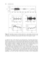
Figure 1.8 Example of speech waveform uttered by a male subject about the word
‘‘problems.’’ The expanded views of a voiced frame and an unvoiced frame are shown, with
the magnitude of the Fourier transorm plotted. The frame is 256 samples in length.
14
INTRODUCTION
technique called linear prediction (Chapter 4), it is possible to estimate the para-
meters of the time-varying filter from the observed signal.
The assumption of the model is that the energy distribution of the speech signal
in frequency domain is totally due to the time-varying filter, with the lungs produ-
cing an excitation signal having a flat-spectrum white noise. This model is rather
efficient and many analytical tools have already been developed around the concept.
The idea is the well-known autoregressive model, reviewed in Chapter 3.
A Glimpse of Parametric Speech Coding
Consider the speech frame corresponding to an unvoiced segment with 256 samples
of Figure 1.8. Applying the samples of the frame to a linear prediction analysis pro-
cedure (Chapter 4), the coefficients of an associated filter are found. This filter has
system function
HðzÞ¼
1

1 þ
P
10
i¼1
a
i
z
Ài
with the coefficients denoted by a
i
, i ¼ 1 to 10.
White noise samples are created using a unit variance Gaussian random number
generator; when passing these samples (with appropriate scaling) to the filter, the
output signal is obtained. Figure 1.10 compares the original speech frame, with two
realizations of filtered white noise. As we can see, there is no time-domain corre-
spondence between the three cases. However, when these three signal frames are
played back to a human listener (converted to sound waves), the perception is
almost the same!
How could this be? After all, they look so different in the time domain. The
secret lies in the fact that they all have a similar magnitude spectrum, as plotted
in Figure 1.11. As we can see, the frequency contents are similar, and since the
human auditory system is not very sensitive toward phase differences, all three
Output speech
White
noise
generator
Time-
varying
filter
Lungs

Trachea
Pharyngeal cavity
Nasal cavity
Oral cavity
Nostril
Mouth
Figure 1.9 Correspondence between the human speech production system with a simplified
system based on time-varying filter.
SPEECH PRODUCTION AND MODELING
15
frames sound almost identical (more on this in the next section). The original
frequency spectrum is captured by the filter, with all its coefficients. Thus, the
flat-spectrum white noise is shaped by the filter so as to produce signals having a
spectrum similar to the original speech. Hence, linear prediction analysis is also
known as a spectrum estimation technique.
0 50 100 150 200 250
−5000
0
5000
0 50 100 150 200 250
−5000
0
5000
0 50 100 150 200 250
−5000
0
5000
n
n
n

s[n]
s1[n]
s2[n]
Figure 1.10 Comparison between an original unvoiced frame (top) and two synthesized
frames.
0 20 40 60 80 100 120
0.1
1
10
100
1ؒ10
3
k
|S[k]|
Figure 1.11 Comparison between the magnitude of the DFT for the three signal frames of
Figure 1.10.
16
INTRODUCTION
How can we use this trick for speech coding? As we know, the objective is to
represent the speech frame with a lower number of bits. The original number of bits
for the speech frame is
Original number of bits ¼ 256 samples Á 16 bits=sample ¼ 4096 bits:
As indicated previously, by finding the coefficients of the filter using linear pre-
diction analysis, it is possible to generate signal frames having similar frequency
contents as the original, with almost identical sounds. Therefore, the frame can
be represented alternatively using ten filter coefficients, plus a scale factor. The
scale factor is found from the power level of the original frame. As we will see later
in the book, the set of coefficients can be represented with less than 40 bits, while
5 bits are good enough for the scale factor. This leads to
Alternative number of bits ¼ 40 bits þ 5 bits ¼ 45 bits:

Therefore, we have achieved an order of magnitude saving in terms of the
number of required bits by using this alternative representation, fulfilling in the
process our objective of bit reduction. This simple speech coding procedure is
summarized below.
 Encoding
Derive the filter coefficients from the speech frame.
Derive the scale factor from the speech frame.
Transmit filter coefficients and scale factor to the decoder.
 Decoding
Generate white noise sequence.
Multiply the white noise samples by the scale factor.
Construct the filter using the coefficients from the encoder and filter the scaled
white noise sequence. Output speech is the output of the filter.
By repeating the above procedures for every speech frame, a time-varying filter
is created, since its coefficients are changed from frame to frame. Note that this
overly simplistic scheme is for illustration only: much more elaboration is neces-
sary to make the method useful in practice. However, the core ideas for many
speech coders are not far from this uncomplicated example, as we will see in later
chapters.
General Structure of a Speech Coder
Figure 1.12 shows the generic block diagrams of a speech encoder and decoder. For
the encoder, the input speech is processed and analyzed so as to extract a number of
parameters representing the frame under consideration. These parameters are
encoded or quantized with the binary indices sent as the compressed bit-stream
SPEECH PRODUCTION AND MODELING
17
(see Chapter 5 for concepts of quantization). As we can see, the indices are packed
together to form the bit-stream; that is, they are placed according to certain prede-
termined order and transmitted to the decoder.
The speech decoder unpacks the bit-stream, where the recovered binary indices

are directed to the corresponding parameter decoder so as to obtain the quantized
parameters. These decoded parameters are combined and processed to generate the
synthetic speech.
Similar block diagrams as in Figure 1.12 will be encountered many times in later
chapters. It is the responsibility of the algorithm designer to decide the functionality
and features of the various processing, analysis, and quantization blocks. Their
choices will determine the performance and characteristic of the speech coder.
1.4 SOME PROPERTIES OF THE HUMAN AUDITORY SYSTEM
The way that the human auditory system works plays an important role in speech
coding systems design. By understanding how sounds are perceived, resources in
the coding system can be allocated in the most efficient manner, leading to
improved cost effectiveness. In subsequent chapters we will see that many speech
coding standards are tailored to take advantage of the properties of the human audi-
tory system. This section provides an overview of the subject, summarizing several
Input
PCM
speech
…
Index 1 Index 2 Index N
Bit-stream
Bit-stream
Index 1 Index 2 Index N
…
Synthetic
speech
Analysis and processing
Extract
enand code
parameter 1
Extract

enand code
parameter 2
Extract
enand code
parameter N
Pack
Unpack
Decode
parameter 1
Decode
parameter 2
Decode
parameter N
Combine and processing
Figure 1.12 General structure of a speech coder. Top: Encoder. Bottom: Decoder.
18
INTRODUCTION