Priority-Lasso: A simple hierarchical approach to the prediction of clinical outcome using multi-omics data
Bạn đang xem bản rút gọn của tài liệu. Xem và tải ngay bản đầy đủ của tài liệu tại đây (1.05 MB, 14 trang )
Klau et al. BMC Bioinformatics (2018) 19:322
/>
METHODOLOGY ARTICLE
Open Access
Priority-Lasso: a simple hierarchical
approach to the prediction of clinical outcome
using multi-omics data
Simon Klau1*
, Vindi Jurinovic1 , Roman Hornung1 , Tobias Herold2 and Anne-Laure Boulesteix1
Abstract
Background: The inclusion of high-dimensional omics data in prediction models has become a well-studied topic in
the last decades. Although most of these methods do not account for possibly different types of variables in the set of
covariates available in the same dataset, there are many such scenarios where the variables can be structured in
blocks of different types, e.g., clinical, transcriptomic, and methylation data. To date, there exist a few computationally
intensive approaches that make use of block structures of this kind.
Results: In this paper we present priority-Lasso, an intuitive and practical analysis strategy for building prediction
models based on Lasso that takes such block structures into account. It requires the definition of a priority order of
blocks of data. Lasso models are calculated successively for every block and the fitted values of every step are included
as an offset in the fit of the next step. We apply priority-Lasso in different settings on an acute myeloid leukemia (AML)
dataset consisting of clinical variables, cytogenetics, gene mutations and expression variables, and compare its
performance on an independent validation dataset to the performance of standard Lasso models.
Conclusion: The results show that priority-Lasso is able to keep pace with Lasso in terms of prediction accuracy.
Variables of blocks with higher priorities are favored over variables of blocks with lower priority, which results in easily
usable and transportable models for clinical practice.
Keywords: Cox regression, Lasso, Multi-omics data, Penalized regression, Prediction model, Priority-lasso
Background
Many cancers are heterogeneous diseases regarding biology, treatment response and outcome. For example, in
the context of acute myeloid leukemia (AML), a variety of classifiers and recommendations were published to
guide treatment decisions [1]. We and others have recently
shown that gene expression markers as well as mutational
profiling are able to improve risk prediction based on
standard clinical markers [2–5]. Other types of biomarkers such as copy number variation data or methylation
data may also be used for this purpose in the future.
However, irrespective of the considered specific end point
(e.g., overall survival, resistant disease, early death) no
model is currently able to precisely predict the outcome
*Correspondence:
Institute for Medical Information Processing, Biometry and Epidemiology,
University of Munich, Munich, Germany
Full list of author information is available at the end of the article
1
of AML patients. To date, the most powerful prognostic models are based on cytogenetics and gene expression
markers [6].
In the present paper, we use the term omics to
denote molecular biomarkers measured through highthroughput experiments. Beyond the example of AML
mentioned above, the integration of multiple types of
omics biomarkers with the aim of improved prediction
accuracy has been a focus of much attention in the past
years, see for example [7] and references therein. While
prediction modelling using a single type of omics markers
is a well-studied topic, it is not clear how different types
of biomarkers should be handled simultaneously when
deriving a prediction model.
In addition to the highly important topic of prediction accuracy, encompassing both discrimination ability
and calibration, clinical reality requires analysts to take
© The Author(s). 2018 Open Access This article is distributed under the terms of the Creative Commons Attribution 4.0
International License ( which permits unrestricted use, distribution, and
reproduction in any medium, provided you give appropriate credit to the original author(s) and the source, provide a link to the
Creative Commons license, and indicate if changes were made. The Creative Commons Public Domain Dedication waiver
( applies to the data made available in this article, unless otherwise stated.
Klau et al. BMC Bioinformatics (2018) 19:322
aspects related to usability into account when developing prediction models for clinical practice. Firstly, a
model including several hundreds/thousands of variables
is much more difficult to implement in clinical practice
than a model including only a handful of variables. Sparsity is thus an important aspect of the model which contributes to its practical utility in clinical settings. Secondly,
a model including variables that are already included in
routine diagnostics — such as genetic alterations as recommended by the European LeukemiaNet (ELN) in the
case of AML [1], or variables that can be easily assessed
such as age or common clinical variables — are more likely
to be accepted by physicians than a model including variables measured with new and/or expensive technologies,
maybe even at the expense of a slightly lower prediction
accuracy. These two points are arguments in favor of models that (preferably) include a small number of variables
selected from particular “favorite” sets of variables — as
opposed to, say, a large number of variables selected from
genome-wide data.
Another aspect related to practical usability is the transportability of a prediction model, i.e. the possibility for
potential users to apply the prediction model to their own
data based on information provided by the model developers [8]. Penalized regression methods yielding sparse
models typically yield better transportable models than
black-box machine learning algorithms [8, 9]. For example, to apply a Lasso logistic regression model [10] for
making predictions for their own patients, users only
need the fitted regression coefficients and names of the
selected variables to compute the score and, if they want
to compute predicted probabilities, the fitted intercept. In
contrast, a prediction tool constructed using, for example, the random forest algorithm, can be applied by other
researchers or clinicians only if they have access to a
software object (such as the output of the R function ‘randomForest’ if the package of the same name is used) or
the dataset and the code used to construct it — which
may become obsolete after a few years. In this sense, Lasso
logistic regression is preferable to random forest as far
as transportability and sustainability are concerned. Note
that model interpretation is also particularly easy with
sparse penalized regression methods.
Finally, coming back to prediction accuracy, we note
that medical experts often have some kind of prior knowledge regarding the information content of different sets
of variables. For example, they often expect (a particular
set of ) the clinical variables to have high prediction ability and a large proportion of the gene expression variables
to be less relevant. Such prior knowledge should ideally be
taken into account while constructing a prediction model.
Motivated by the need, in the context of AML research
and other fields, for sparse transportable models selecting
preferably variables that are easy to collect or expected to
Page 2 of 14
yield good prediction accuracy, we suggest priority-Lasso,
a simple Lasso-based approach. Priority-Lasso is a hierarchical regression method which builds prediction rules
for patient outcomes (e.g., a time-to-event, a response status or a continuous outcome) from different blocks of
variables including high-throughput molecular data while
taking clinicians’ preference into account. More precisely,
clinicians define “blocks” of variables (which may simply
correspond to the type of data, e.g., the block of methylation variables or the block of gene expression variables)
and order these blocks according to their level of priority.
The prediction model is then fitted in a stepwise manner:
In turn, each block of variables is considered as a covariate matrix in Lasso regression, in the sequence of priority
specified by the clinician; see the “Methods” section for
more details.
The priority-Lasso procedure is fast and simple. It can
cope with all the types of outcome variables accepted by
Lasso and, more generally, inherits its properties. The
hierarchical principle of priority-Lasso can essentially also
be applied to extensions of Lasso, including but not limited to elastic net [11], adaptive Lasso [12] or stability
selection [13], but also, more generally, to other prediction methods applicable to high-dimensional covariate
data. Last but not least, note that the priority sequence
imposed by the clinician merely determines which blocks
are prioritized over other blocks with respect to rendering
predictive information that is contained in several blocks.
Predictive information of blocks with low priority that is not
contained in blocks with high priority is still exploited by
priority-Lasso (see “Principles of priority-Lasso” section
for details).
The rest of this paper is structured as follows. Section
“Methods” presents the priority-Lasso method and its
implementation in detail. In “Results” section, the method
is illustrated with different settings through an application
to AML data and compared to standard Lasso in terms
of accuracy and included variables. The considered outcome is the survival time and the considered types of data
are comprised of clinical data, the mutation status of several genes and gene expression data. Most importantly,
prediction models are fitted on a training dataset and subsequently validated on an independent dataset following
the recommendations by Royston and Altman [14].
Methods
We first provide a non-technical introduction into the
principles of priority-Lasso in “Principles of priority-Lasso”
section to make these concepts accessible to readers
without strong statistical background and to give a succinct overview. We present the method formally in
“Formalization of priority-Lasso” section, treat its implementation in “R package prioritylasso” section, and
describe in “Validation” section the validation strategy
Klau et al. BMC Bioinformatics (2018) 19:322
inspired from Royston and Altman [14] adopted in our
illustrative example.
Principles of priority-Lasso
Priority-Lasso is a method that can construct a prediction
model for a clinical outcome of interest (e.g., a time to
event or a response status and continuous outcome) based
on candidate variables, using an available training dataset.
Before running priority-Lasso, the user is required to first
specify a block structure for the covariates where each
covariate belongs to exactly one of M blocks and, second,
a priority order of these blocks.
A block may be of a particular data type, for example
“clinical data”, “gene expression data” or “methylation data”,
but the classification of variables into blocks may also be
finer. For example, clinical data may be divided into two
blocks, e.g., the demographic data (e.g., age or sex) in a
first block and clinical data related to the tumor in the
second block. Once the blocks of variables are defined,
the clinician orders them according to their level of priority. High priority should be given to blocks which are
easy and/or inexpensive to collect or are already routinely
collected in clinical practice.
After this definition, the prediction model is fitted in a
stepwise manner. In the first step, a Lasso model is fitted
to the block with highest priority. The goal of this step is
simply to explain the largest possible part of the variability
in the outcome variable by the covariates from the block
with highest priority. In the second step, a Lasso model is
fitted to the block with second highest priority using the
linear score from the first step as an offset, i.e., this linear
score is forced into the model with coefficient fixed to 1.
In the special case of a metric outcome, this corresponds
to fitting a second Lasso model (without the offset) to the
residuals from the first Lasso model using the block with
second highest priority as covariate matrix. The goal of
this second step is thus to use the variables from the second block to explain remaining variability in the outcome
variable that could not be explained by covariates from the
first block.
In the third step, a Lasso regression is fitted to the
block with third highest priority using the linear score
from the second step as offset. The special case of a
metric outcome is correspondingly equivalent to fitting
a Lasso model to the residuals from the second Lasso
model using the block with third highest priority. This
procedure is iterated until all blocks have been considered in turn. Thus, in the case of a metric outcome, at
each step the current block is fitted to the residuals of
the previous step. Generalizing to other types of outcome variables, in each step the current block is fitted
to the outcome conditional on all blocks with higher priority that were considered in the previous steps. In this
way, blocks of variables with low priority enter the model
Page 3 of 14
only if they explain variability that is not explainable by
blocks with higher priority. Compared to non-hierarchical
approaches, priority-Lasso tends to yield models in which
variables from the most prioritized blocks play a more
important role.
This procedure was motivated by the fact that there
is frequently a strong overlap of predictive information
across the considered blocks. For example, some gene
expression and gene mutation variables can be associated with the same phenotype, which is why these two
different types of omics data may contain similar predictive information. Moreover, clinical covariates and omics
covariates often carry similar predictive information. If, in
priority-Lasso, a block A is given a higher priority than a
block B, this means that the part of the predictive information contained in A and B that is common to both blocks
will be obtained from block A. The larger the number
of blocks, the lower the information contained in individual blocks, that is not contained in any other block.
Thus, in the presence of a large number of blocks there
is a high chance that priority-Lasso will exclude variables
from blocks of low priority, because the predictive information contained therein may also be contained in the
data of blocks of higher priority. Therefore, by providing
a priority sequence, the analyst can decide which blocks
should be prioritized over others with respect to providing
predictive information redundant among blocks. The chosen priority sequence can, however, be expected to have
a limited impact on the prediction error for the following reason: If a block A with strong predictive power is
attributed a low priority, its predictive power will nevertheless be exploited in the prediction rule. This is because
the proportion of the variability of the outcome variable
that is only explainable by block A will still be unexplained
before block A is considered as a covariate block in the
iterative procedure.
Formalization of priority-Lasso
In the following description, we consider M blocks of continuous or binary variables that are all to be penalized,
and a continuous outcome variable for the sake of simplicity. Extensions to time-to-event and binary outcomes
are straightforward using the corresponding variants of
Lasso (Cox Lasso and logistic Lasso, respectively, see [15]
and [10, 16]). The extension to multicategorical variables
is also straightforward using an appropriate coding of the
variables.
Let xij denote the observed value of the jth variable (j =
1, . . . , p) for the ith subject (i = 1, . . . , n) and yi denote the
observed outcome of subject i. For simplicity it is assumed
that each variable is centered to have mean zero over the n
observations. The standard Lasso method [10] estimates
the regression coefficients β1 , . . . , βp of the p variables by
minimizing the expression
Klau et al. BMC Bioinformatics (2018) 19:322
n
⎛
p
⎝yi −
i=1
⎞2
p
xij βj ⎠ + λ
j=1
Page 4 of 14
|βj |
j=1
with respect to β1 , . . . , βp , where λ is a so-called penalty
parameter. This method performs both regularization
(shrinkage of the estimates) and variable selection (i.e.,
some of the estimates are shrunken to zero, meaning that
the variable is excluded from the model). The amount of
shrinkage is determined by the parameter λ, which is considered as a tuning parameter of the method and is in
practice most often chosen using cross-validation.
We now adapt our notation to the case of variables
forming groups that is considered in this paper. From now
on, the observations of the pm variables from block m for
(m)
subject i are denoted as x(m)
i1 , . . . , xipm , for i = 1, . . . , n
and m = 1, . . . , M. The number of blocks M usually
ranges from 2 to, say, 10 in practice, while the number
pm of variables often varies strongly across the blocks.
For example, blocks of clinical variables typically include a
very small number of variables, say, pm ≈ 10, while blocks
of molecular variables from high-throughput experiments
may include several tens or hundreds of thousands of
variables.
(m)
denotes the
Similarly to the definition of x(m)
ij , βj
regression coefficient of the jth variable from block m,
(m)
for j = 1, . . . , pm , while βˆj
stands for its estimated
counterpart.
Let us further denote as π = (π1 , . . . , πM ) the permutation of (1, . . . , M) that indicates the priority order: π1
denotes the index of the block with highest priority, while
πM is the index of the block with the lowest priority. For
example, if M = 4, π = (3, 1, 4, 2) means that the third
block has highest priority, the first block has second highest priority, and so on. Conversely, the priority level of a
given block is indicated by the position of its index in the
vector π .
In the first step of priority-Lasso, the variables from
block π1 are used to fit a Lasso regression model. The
(π )
(π )
coefficients β1 1 , . . . , βpπ11 are estimated by minimizing
⎛
⎞2
n
i=1
⎝yi −
pπ1
(π ) (π )
xij 1 βj 1 ⎠
(π1 )
pπ1
j=1
(π1 )
βj
+λ
.
(π )
(π )
βˆ1 1 , . . . , βˆpπ11 , which are then used to calculate ηˆ 1,i (π).
This overoptimism is essentially similar to the well-known
overoptimism that results from estimating the prediction
error of a prediction rule using the observations in the
training dataset. When using this over-optimistic estimate
ηˆ 1,i (π) as an offset in the second step, the influence of
block π2 conditional on the influence of block π1 will
tend to be underestimated. The reason for this is that
by considering the over-optimistic estimate ηˆ 1,i (π) as an
offset, a part of the variability in yi is removed that is
actually not explainable by block π1 but would possibly
be explainable by block π2 . As noted above, this problem
results from the fact that yi is contained in the train(π )
(π )
ing data used for estimating β1 1 , . . . , βpπ11 . As a solution
to this problem we suggest estimating the offsets η1,i (π)
using cross-validation in the following way: 1) Split the
dataset S randomly into K approximately equally sized
parts S1 , . . . , SK ; 2) For k = 1, . . . , K: obtain estimates
(π1 )
(π1 )
βˆS\S
, . . . , βˆS\S
of the Lasso coefficients using the
k ,1
k ,pπ1
training data S \ Sk and for all i ∈ Sk (k = 1, . . . , K),
calculate the cross-validated offsets as
(π )
(π ) (π )
(π )
ηˆ 1,i (π ) = βˆ1 1 xi1 1 + . . . + βˆp(ππ 1 ) xipπ1 .
1
1
In “Principles of priority-Lasso” section we noted that
this linear predictor is used as an offset in the second
step in which we fit a Lasso model to block π2 . However,
the linear score ηˆ 1,i (π ) tends to be over-optimistic with
respect to the information usable for predicting yi that is
contained in block π1 . The reason for the latter is that
yi was part of the data used for obtaining the estimates
(π )
(π )
1
1
In the second step the coefficients of the variables in
block π2 are thus estimated by minimizing
⎛
⎞2
n
⎝yi − ηˆ 1,i (π)CV −
i=1
pπ2
2 ) (π2 ) ⎠
x(π
+λ(π2 )
ij βj
j=1
pπ2
βj(π2 ) .
j=1
(π ) (π )
(π ) (π )
Using ηˆ 2,i (π) = ηˆ 1,i (π)CV + βˆ1 2 xi1 2 + . . . + βˆpπ22 xipπ2 as
2
an offset in the third step in which we fit a Lasso model to
block π3 could again lead to underestimating the influence
of block π3 conditional on the influences of blocks π1 and
π2 . This is because, analogously to the first step, the esti(π )
(π )
mates βˆ1 2 , . . . , βˆpπ22 used to calculate ηˆ 2,i (π ) are overly
well adapted to the residuals yi − ηˆ 1,i (π)CV . Therefore,
we again suggest to calculate cross-validated estimates,
ηˆ 2,i (π)CV , of the offsets analogously to the first step.
Priority-Lasso proceeds analogously for the remaining
groups until the final (Mth) fit, where the following linear
predictor is obtained:
j=1
The linear predictor fitted in step 1 is given as
(π )
ηˆ 1,i (π)CV = βˆS\S1k ,1 xi1 1 + . . . + βˆS\S1k ,pπ xipπ1 .
M pπm
ηˆ M,i (π ) =
βˆj(πm ) xij(πm ) .
m=1 j=1
Note that when the offsets are not estimated by crossvalidation but the estimates ηˆ 1,i (π), . . . , ηˆ M−1,i (π) are
used, the effects described above of underestimating the
conditional influences of the individual blocks accumulate. Thus, the influences of blocks with higher priority are
underestimated to a less stronger degree than are blocks
with low priority. This could eventually lead to the exclusion of blocks with lower priority that are valuable for
Klau et al. BMC Bioinformatics (2018) 19:322
prediction. This is particularly problematic in cases in
which low priorities are attributed to blocks with high predictive information. Thus, cross-validated offsets may be
used to avoid suboptimal models that may result in cases
in which the priority sequence does not attribute high
priority to blocks with high predictive power. Note, however, that we are not interested in determining priority
sequences that perform optimally from a statistical point
of view. Instead, the priority sequence reflects the specific
needs of the user, who particularly cares about practicability. Notwithstanding the above mentioned advantages of
using cross-validated offsets, we nevertheless also include
the version of priority-Lasso without cross-validated offsets in our application study (see “Results” section) for
several reasons. Firstly, because the version with crossvalidated offsets is more computationally intensive, and
thus might not be easily applicable in all situations. Secondly, we aim to illustrate that this version tends to
accredit more influence to the blocks with lower priority
than does the version without cross-validated offsets. In
addition, the suspected tendency of the version without
cross-validated offsets to exclude blocks with lower priority might be advantageous in applications in which these
blocks contain data types that are expensive to collect or
not well established.
R package prioritylasso
The priority-Lasso method (for continuous, binary, and
survival outcomes) is implemented in the function ‘prioritylasso’ from our new R package of the same name
(version 0.2), which is publicly available from the “Comprehensive R Archive Network” repository. This package
uses the implementation of Lasso regression provided by
the R package ‘glmnet’ (see [17], and for the special case of
Cox-Lasso, see [18]).
The M penalty parameters λ(π1 ) , . . . , λ(πM ) are chosen
via cross-validation in the corresponding steps. As in ‘glmnet’, two variants are implemented: The penalty parameter
can be chosen either in such a way that the mean crossvalidated error is minimal (denoted as ‘lambda.min’), or
in such a way that it yields the sparsest model with error
within one standard error of the minimum (denoted as
‘lambda.1se’). The latter option yields sparser models. In
order to further enforce sparsity at the convenience of
the clinician, our package allows to specify a maximum
number of non-zero coefficients for each block.
Furthermore, the function ‘prioritylasso’ offers the
option to leave the block with highest priority unpenalized
(i.e., to set λ(π1 ) to 0), provided the number of variables pπ1
in this group is smaller than the sample size n. Depending on the outcome, the estimation is then performed via
generalized linear regression or via Cox regression [19].
Another variant of the priority-Lasso method is implemented in the function ‘cvm_prioritylasso’, which makes
Page 5 of 14
it possible to take more than one vector π as the input
and choose the best one through minimizing the crossvalidation error. This variant is useful in cases where it
makes sense to take the group structure into account but
the clinician does not feel comfortable assigning clear-cut
priorities to each of the groups.
Note that our package solely aims at building prediction models with different types of already prepared omics
data available as an n × p data matrix. However, generating such multi-omics data matrices from several types of
raw data files requires considerable effort. We refer to Bioconductor software packages [20] that allow convenient
annotation and organization of multi omics data. As an
important example, the ‘MultiAssayExperiment’ data class
[21] can be used for data preparation prior to running
‘prioritylasso’.
Validation
In “Results” section, we apply the priority-Lasso method
as well as the classical Lasso to fit prediction models for a
time-to-event on a training dataset and subsequently evaluate these models on a validation dataset; see “AML data”
section for a description of the data used in this analysis.
The present section briefly describes the criteria considered to assess prediction accuracy and the procedures
used for validation of the considered models, following
the recommendations of Royston and Altman [14]. These
authors emphasize in their paper that validation comprises both discrimination and calibration. Hence, we
perform both in our analysis and focus on the methods
denoted as methods 3, 4, 6, and 7 in their paper.
Firstly, following method 3, we present some measures
of discrimination. Instead of Harrell’s C-index, a common measure to quantify the goodness of fit, we show
the results of the Uno’s C-index [22], an adapted version
of Harrell’s C-index that accounts for censored data and
is thus more appropriate in our context. Another useful
measure is the integrated Brier score [23] assessing both
calibration and discrimination simultaneously, which we
calculate over two different time spans: up to two years
and up to the time of the last event. To visualize the
results, we also show the corresponding prediction error
curves obtained using the R package ‘pec’ [24].
Secondly, following method 4 of Royston and Altman
[14], we display Kaplan-Meier curves that can be useful
for both discrimination and calibration. For each considered prediction model, we define three risk groups, which
corresponds to standard practice in the AML context. See
for example the newest European Leukemia Net (ELN)
genetic risk stratification of AML, which classifies patients
into a low-, intermediate-, and a high-risk group [1] and
will be referred to as ELN2017 score in the sequel. To build
three groups based on a considered score, we choose the
two cutpoints that yield the highest logrank statistic in the
Klau et al. BMC Bioinformatics (2018) 19:322
training data. We then present the Kaplan-Meier curves
of the three risk groups for both training and validation
sets. Good separation of the three curves in the validation
dataset indicates good discrimination.
These three Kaplan-Meier curves observed for the validation dataset can also be compared to the predicted
curves for the three risk groups in the validation dataset
(Royston and Altman’s method 7). By “predicted curve
for a risk group”, we mean the average of the individual
predicted curves of the patients within this risk group.
Good agreement between observed and predicted curves
suggests good calibration. Thirdly, as an extension of the
graphical check for discrimination, we also examine the
hazard ratios across risk groups (Royston and Altman’s
method 6).
Beyond these methods, we report the AUC, the true
positive rate (TPR, also known as sensitivity) and the true
negative rate (TNR, also known as specificity) of each
score at two years after the diagnosis. This time point
was chosen because its ratio of cases to survivors is the
closest to 1. The true positive and the true negative rate
are calculated with the median of each score as a cutoff
for categorizing the scores into two groups. Furthermore,
we consider a modified version of Royston and Altman’s
method 1. They suggest performing a regression with the
linear predictor from the model as the only covariate. For
a standard Cox model the resulting coefficient is exactly
1 in the training data and should be approximately 1 in
the validation data to indicate a good model fit. However, since we perform penalized regression this method
is not applicable to our model. Therefore, we modify this
criterion in calculating the calibration slopes in both training and validation data. The difference between the slope
obtained using the training data and the one obtained
using the validation data is a measure for the extent of the
overoptimistic assessment of discrimination ability that is
obtained using the training data.
Results
The section starts with a brief description of the
AML example dataset (“AML data” section). Then
we present four models fitted using priority-Lasso
(“Results of priority-Lasso” section) and compare them
with the current clinical standard model and with
two models fitted through standard Lasso (i.e., without taking the block structure into account) in terms of
included variables (“Assessing included variables” section)
and performance in the independent validation data
(“Assessing prediction accuracy” section). These models
are all fitted with a restricted number of selected variables.
The same models without restrictions to the number of
variables are presented in Additional file 1 for further
comparisons. The complete R code written to perform the
analyses is available from Additional file 2.
Page 6 of 14
AML data
In this study we use two independent datasets, denoted
training set and validation set hereafter, including variables belonging to different blocks (see details below).
All patients included in the analysis received cytarabine
and anthracycline based induction treatment. The training set consists of 447 patients randomized and treated
in the multicenter phase III AMLCG-1999 trial (clinicaltrials.gov identifier NCT00266136) between 1999 and
2005 [25, 26]. The patients are part of a previously
published gene expression dataset (GSE37642) analyzed
with Affymetrix arrays [27]. All patients with a t(15;17)
or myelodysplastic syndrome are excluded, as well as
patients with missing data.
The validation set consists of all patients with
available material treated in the AMLCG-2008 study
(NCT01382147) [28], a randomized, multicenter phase III
trial (n = 210) and additional n = 40 patients that had
resistant disease and were treated in the AMLCG-1999
trial. The dataset is publicly available at the Gene Expression Omnibus repository (GSE106291). The detailed
inclusion and exclusion criteria were described previously
[29]. The patients of the validation set were analyzed
by RNAseq. For comparability, all continuous variables
are standardized to a mean zero and variance one. All
study protocols are in accordance with the Declaration of
Helsinki and approved by the institutional review boards
of the participating centers. All patients provided written
informed consent for inclusion on the clinical trial and
genetic analyses.
Results of priority-Lasso
We apply priority-Lasso on the training dataset (n = 447,
described in “AML data” section), considering four
different scenarios. These scenarios differ in the way
the score ELN2017 is included in the analysis and
whether or not the offsets are cross-validated (see
“Formalization of priority-Lasso” section). Furthermore,
we always apply the ‘lambda.min’ procedure and 10-foldcross-validation for the choice of the penalty parameter
in each step. However, since prediction performance is
not the main concern in our analyses, the ‘lambda.1se’
approach would also be a reasonable option. In
“Sensitivity analysis” section we show some results with
‘lambda.1se’ in addition to our main analyses. Furthermore, we allow for a maximum of 10 gene expression
variables for each scenario as we want to keep the
resulting model as simple as possible and experience
has shown that in survival prediction for AML patients
only a few gene expression values have a considerable
influence on the outcome. Moreover, gene expression
values are not easy to implement in clinical routine.
We define the following blocks and corresponding
priorities:
Klau et al. BMC Bioinformatics (2018) 19:322
• Block of priority 1: the score ELN2017 [1]. It can be
represented in different ways which are explained in
the definition of the scenarios.
• Block of priority 2: 8 clinical variables measured at
different scales
• Block of priority 3: 40 binary variables, each of which
represents the mutation status for a certain gene
• Block of priority 4: 15809 continuous variables, each
of which is the expression value of a certain gene
The order of these blocks have been determined by a
physician involved in the project, who has many years
of experience in the treatment of patients with AML,
as well as experience with AML outcome prediction.
These choices are based on practical considerations.
However, alternative block orders could be reasonable
from other points of view. For example, if the focus is
solely on the maximization of prediction performance
without any practical constraints, we refer to the function ‘cvm_prioritylasso’ from our R package ’prioritylasso’
which chooses the best order of blocks from two or more
priority options according to the mean cross-validated
performance. In addition to our main analyses that are
based on an ordering that takes practical aspects into
account as outlined above, we present additional results
obtained for other block orders in “Sensitivity analysis”
section.
Scenario pl1A
In the first scenario, the block of priority 1 consists
of the three-categorical ELN2017 score represented by
two dummy variables. We do not penalize this block
and do not use cross-validated offsets. In this scenario
the selected model includes only 7 variables represented
by 8 coefficients: the dummy variables ELN2017_2 and
ELN2017_3, equaling 1 for the intermediate and the highrisk category, respectively, and 0 otherwise, are selected
by definition, because they result from a fit of a standard Cox model without penalization. Moreover, age, the
Eastern Cooperative Oncology Group performance status (ECOG) [30], white blood cell count (WBC), lactate
dehydrogenase serum level (LDH), hemoglobin level (Hb)
and platelet count (PLT) are selected. The selected variables and their coefficients are displayed in the second and
third column of Table 1. Variables from blocks with priority 3 (mutation status of 40 genes) and 4 (gene expression)
are absent from the model, yielding a particularly sparse
model based on variables which are easy to access.
Scenario pl1B
This scenario is very similar to pl1A with the difference that the offsets are cross-validated as described in
“Formalization of priority-Lasso” section. Because there
are no offsets in the first step of the model fit, the
Page 7 of 14
Table 1 Variables selected by priority-Lasso in scenarios pl1A
and pl1B
Block
Variable
Coef. pl1A
Coef. pl1B
1
ELN2017_2
0.8552
0.8552
ELN2017_3
1.4324
1.4324
2
4
Age
0.3540
0.3556
ECOG (> 1)
0.2794
0.2768
WBC
0.1029
0.1019
LDH
0.1744
0.1763
Hb
0.0529
0.0532
PLT
-0.0788
-0.0800
PHGDH
0.1242
FAM171B
0.0726
SH3PXD2B
0.0192
F12
0.0097
CD109
0.0599
FAM92A1
0.0193
LAPTM4B
0.0079
FAM24B
0.0378
DDIT4
0.0424
DOCK1
0.0295
Column 1: priority of the block the variables are included in. Column 2: variable
name. Column 3 and 4: coefficient of the variable in the Cox Lasso model
coefficients of pl1A and pl1B are the same for the block
of priority 1 (see Table 1, column 4). For the block of
priority 2, the same variables are selected with small
differences in their coefficients. While both models do
not select variables from the block of priority 3, model
pl1B additionally includes 10 gene expression markers—
all with only small influence though. Nevertheless, the fact
that gene expression markers are included in the model
with cross-validated offsets, but not in the model without
cross-validated offsets, illustrates the conjecture made in
“Formalization of priority-Lasso” section: When using the
priority-Lasso version with cross-validated offsets, more
influence tends to be accredited to the blocks with lower
priority compared to when using the version without
cross-validated offsets.
Scenario pl2A
As an alternative approach, considered as sensitivity analysis in the present paper, one may also replace ELN2017
with the 19 variables that are used for its calculation.
Because of the far higher number of variables, we penalize this block of priority 1. The results of the scenario
without cross-validated offsets (scenario pl2A) are displayed in the third column of Table 2, showing that 14
of these 19 variables are selected. While the selected
variables from block 2 are almost the same as in scenario pl1A (except the additional inclusion of sex), now
Klau et al. BMC Bioinformatics (2018) 19:322
Page 8 of 14
Table 2 Variables selected by priority-Lasso in scenarios pl2A
and pl2B
Block
Variable
1
t(8;21)(q22;q22)
-1.0289
-1.0289
inv(16)(p13.1q22)
-1.5444
-1.5444
2
4
Coef. pl2A
Coef. pl2B
NPM1 mut/FLT3-ITD neg or low
-1.0181
-1.0181
biCEBPA
-1.2240
-1.2240
Scenario pl2B
Analogously to scenarios pl1A and pl1B, scenario pl2B is
the same as pl2A, except that the offsets are calculated
with cross-validation. Column 4 of Table 2 contains the
results from this model, showing only small differences in
the block of priority 2, but again large differences in the
selected gene expression markers.
NPM1 wt/FLT3-ITD pos or low
-0.4358
-0.4358
Assessing included variables
t(9;11)(p21;q23)
0.4635
0.4635
For assessing the fitted models with respect to the selected
variables, we consider as a reference two standard Lasso
models fitted to the training data using the whole set of
variables without taking any block structure into account.
The two models differ in the way ELN2017 is treated.
In the first Lasso model (variant ‘Lasso1’) it is considered as the score represented by two dummy variables. In
the second Lasso model it is represented by the 19 variables which are used for its definition (variant ‘Lasso2’).
In order to allow for a fair comparison, we again use
the ‘lambda.min’ procedure and 10-fold-cross-validation
to choose the penalty λ. Moreover, we allow the selection
of a maximum number of variables equal to the number
of all variables in blocks 1-3 for priority-Lasso plus 10.
This corresponds to the fact that we did not restrict the
number of variables of blocks 1-3 for priority-Lasso, but
set the maximum number of gene expression variables
to 10. The resulting models (not shown) clearly select
more variables than the models obtained with priorityLasso. Especially the number of gene expression variables
is much higher (43 for Lasso1 and 52 for Lasso2), whereas
only age for both models and ELN2017_3 for Lasso1
are selected variables from other types of data. Hence,
priority-Lasso favors variables from blocks with high priority compared to standard Lasso and yields models that
include considerably less variables.
Other aberrations
-0.4376
-0.4376
KMT2A rearrangements
-0.5440
-0.5440
Complex karyotype
0.2970
0.2970
Monosomal karyotype
0.0313
0.0313
NPM1 wt/FLT3-ITD pos
0.1712
0.1712
RUNX1 mutations
0.3065
0.3065
ASXL mutations
-0.1224
-0.1224
TP53 mutations
0.4306
0.4306
Age
0.2957
0.2617
Sex
-0.1011
ECOG (> 1)
0.3147
0.3206
WBC
0.0990
0.0589
LDH
0.1681
0.2371
Hb
0.0700
0.0671
PLT
-0.0960
-0.0578
0.0025
ZBTB37
0.0047
MFI2
0.0090
SH3PXD2B
0.0013
PDK3
-0.0187
FAM24B
0.0248
SIK3
-0.0063
OR7A17
0.0039
TBC1D17
-0.0172
0.0418
Assessing prediction accuracy
PHGDH
0.0488
FAM171B
0.0134
FGD5
0.0359
F12
0.0238
IRX1
-0.0090
FAM92A1
0.0239
DDIT4
0.0769
HSPA2
0.0169
Column 1: priority of the block the variable is included in. Column 2: variable name.
Column 3 and 4: coefficient of the variable in the Cox Lasso model. Variables from
the block of priority 4 also appearing in Table 1 are marked in bold
there are 8 gene expression variables selected from
the block of priority 4. We can see that these gene
expression variables are not necessarily the same as in
scenario pl1B.
In order to compare the different approaches we follow
the procedures described in “Validation” section − the
results are shown in Table 3. It can be seen that pl1A
and pl1B reach the highest sensitivity among the scenarios (0.672), whereas especially the raw ELN2017 score is
associated with a far lower value (0.556). In contrast, the
specificity is 0.723 for ELN2017, whereas all other scenarios are associated with a specificity between 0.64 and 0.67.
However, these results represent only one of many possible time points and cutoffs, so their use is doubtful in our
context. The other measures − the AUC, the C-indices,
and the integrated Brier score − do not show great differences across the scenarios either. Only ELN2017 is an
exception with considerably poorer results. For the AUC,
pl1B yields the best result with a value of 0.731, but scenarios pl2B, Lasso1 and Lasso2 are not far worse. For CUno ,
the highest value is 0.664, which is reached by pl2B. The
Klau et al. BMC Bioinformatics (2018) 19:322
Page 9 of 14
Table 3 Validation results for the model scenarios with restrictions to the number of selected variables
pl1A
pl1B
Lasso1
pl2A
pl2B
Lasso2
ELN2017
TPR
0.672
0.672
0.651
0.640
0.658
0.643
0.556
TNR
0.667
0.658
0.661
0.647
0.664
0.653
0.723
AUC
0.711
0.731
0.726
0.713
0.727
0.725
0.663
CUno
0.653
0.660
0.658
0.658
0.664
0.656
0.619
IBS2
0.175
0.172
0.176
0.175
0.172
0.177
0.181
IBS4.4
0.197
0.192
0.191
0.197
0.191
0.193
0.204
Optimism
0.393
0.289
0.920
0.377
0.243
0.984
CILlower
0.339
0.304
0.247
0.387
0.327
0.177
0.418
HRL
0.536
0.455
0.363
0.605
0.566
0.286
0.669
CILupper
CIHlower
HRH
0.849
0.652
0.535
0.946
0.981
0.461
1.074
1.175
1.098
0.948
1.515
1.534
0.974
1.314
1.751
1.651
1.385
2.208
2.199
1.386
1.954
CIHupper
2.612
2.483
2.022
3.216
3.151
1.972
2.907
p-valueLR
1.11e-08
1.05e-8
2.22e-10
1.07e-08
1.74e-08
4.99e-11
1.36e-07
The acronyms in the first column are: TPR: True positive rate; TNR: True negative rate; AUC: Area under the curve, CUno : Uno’s C-index, IBS2 : Integrated Brier score up to 2 years,
IBS4.4 : Integrated Brier score up to 4.4 years, Optimism: difference between calibration slopes of training and validation data, CILlower : lower bound of the 95% confidence
interval for the hazard ratio of the low risk group, HRL : hazard ratio of the low risk group, CILupper : upper bound of the 95% confidence interval for the hazard ratio of the low
risk group, CIHlower : lower bound of the 95% confidence interval for the hazard ratio of the high risk group, HRH : hazard ratio of the high risk group, CIHupper : upper bound of the
95% confidence interval for the hazard ratio of the high risk group, p-value: p-value of the likelihood ratio test
integrated Brier score is calculated over two different time
spans (up to 2 years and up to 4.4 years, the latter being
the time to the last event). After two years, the priorityLasso fit with cross-validated offsets is better than the
other models − no matter how ELN2017 is treated. Over
the whole time period, Lasso1 and pl2B give the lowest IBS, followed by Lasso2, indicating a lower prediction
error for the Lasso models in the second half of the whole
time period. This can also be observed in Fig. 1. Scenarios pl1B and pl2B perform best in the first two years but
they are outperformed by Lasso afterwards. As expected,
priority-Lasso with cross-validated offsets is always better
than without. All fitted models are associated with a much
lower prediction error than ELN2017 alone. The results
from the prediction error curves do not differ substantially between the two panels of Fig. 1, that is, they are
robust with regard to the handling of ELN2017.
The Kaplan-Meier curves for training and validation
data are shown in Fig. 2. The discrimination by Lasso
is obviously very good in the training data, but worse
in the validation data. Especially the difference in survival between intermediate and high risk is not very
clear. For both representations of ELN2017, the priorityLasso models with and without cross-validated offsets feature a similar discrimination, where, however, the results
obtained using the version with cross-validated offsets are
slightly better. For the scenario with all ELN2017 variables, the priority-Lasso models give the best results in the
validation data among all scenarios. In contrast, ELN2017
discriminates less well between the three risk groups. The
results concerning Lasso indicate systematic overfitting
in the training data. This is consistent with the results
seen in “Assessing included variables” section where Lasso
included much more variables than the other methods. It
can also be seen from the row ‘optimism’ of Table 3. The
difference of the slopes between training and validation
data is the largest for the Lasso models, indicating that this
method is associated with the highest overoptimism.
A possible way of quantifying the results seen in Fig. 2
is to consider the hazard ratios across risk groups in the
validation set as shown in the lower half of Table 3. The
intermediate group serves as a baseline here. The result of
the likelihood ratio test is significant for all models. The
discrimination between low and intermediate group is
worst for the ELN2017 score. As already seen in Fig. 2, the
discrimination between the low and intermediate group is
better for Lasso than priority-Lasso. In contrast, priorityLasso has a higher hazard ratio for the high risk group, in
particular when using all ELN variables. These observations are also consistent with the results shown in Fig. 1,
where the prediction was better for priority-Lasso than for
Lasso in the earlier years, but worse in the later years. This
corresponds to better prediction for shorter survival times
and worse prediction for longer survival times, respectively. The fact that ELN2017 is included in the results of
priority-Lasso, but not standard Lasso except ELN2017_3
in Lasso1, also seems to play a role for this issue. Both
Fig. 2 and the hazard ratios clearly show that the prediction is better for high risk groups than for low risk groups
with the raw ELN2017 score.
Klau et al. BMC Bioinformatics (2018) 19:322
Page 10 of 14
Fig. 1 Prediction error curves. The curves show the Brier scores calculated in the validation data for the different scenarios and for different time
points. The left panel contains the models considering ELN2017 as categories. The right panel contains the models considering all ELN variables. The
Reference scenario results from the Kaplan-Meier estimation and is the same in both panels. Furthermore, curves for ELN2017, for priority-Lasso with
and without cross-validated offsets, and for standard Lasso are shown
Finally, we present the Kaplan-Meier curves for calibration in Fig. 3. For all the scenarios there are groups that
reveal some miscalibration. For the Lasso models, especially the high risk groups differ between predicted and
observed validation curves. The scenarios pl2A and pl2B
show more differences between predictions and observations in the low risk groups than the other scenarios—the
same fact applies to pl1A and pl1B in the intermediate risk
group.
Sensitivity analysis
In order to investigate the influence of different block
orders on the selected variables, we run the four different
scenarios of priority-Lasso with every possible block order
(data not shown). The results show that the block order
can have substantial influence on the number of selected
variables. For the scenarios pl1A and pl1B, sparsest models are obtained with our priority definition, illustrating
that priority-Lasso takes advantage of prior knowledge.
Higher numbers of variables are obtained for other block
orders with maximum values of 45 (pl2A, π = (4, 3, 1, 2)
and π = (4, 3, 2, 1)). Seven of the eight selected variables
in pl1A are chosen for almost every scenario of priorityLasso and block orders, demonstrating their importance
even in blocks of low priority. Remarkably, only a small
part of them are found in the standard Lasso models (age
in Lasso1 and Lasso2, as well as ELN2017_3 in Lasso1).
It can be further observed that many of the selected gene
expression variables are selected for only a small fraction
of models.
In additional sensitivity analyses we consider the four
scenarios with the ‘lambda.1se’ setting in order to
choose the M values λ(π1 ) , . . . , λ(πM ) as discussed in
“R package prioritylasso” section. As expected, the
‘lambda.1se’ setting leads to a smaller number of selected
variables for all scenarios. In total, the number of variables
is 4, 10, and 15 for priority-Lasso with ELN categories,
priority-Lasso with ELN variables (both with and without cross-validated offsets), and Lasso, respectively. The
four different priority-Lasso models solely select variables
from blocks 1 and 2. On the other hand, apart from age,
Lasso selects only gene expression variables.
Discussion
We introduced priority-Lasso, a simple Lasso-based intuitive procedure for patient outcome modelling based on
blocks of multiple omics data that incorporates practical
constraints and/or prior knowledge on the relevance of
the blocks. The procedure essentially inherits most properties of Lasso. Its basic principle is however not limited
to Lasso and could be easily adapted to recently developed
variants of penalized regression.
Klau et al. BMC Bioinformatics (2018) 19:322
Page 11 of 14
Fig. 2 Kaplan-Meier curves for training and validation data in three risk groups. The three risk groups were built according to the highest logrank
statistic in the training data. The left panel contains the results for the standard Lasso models and the raw ELN2017 score. The middle and right
panels contain the plots of priority-Lasso with and without cross-validated offsets, respectively. The top and middle panels show the results
considering ELN2017 as categories and using all ELN variables, respectively
An important feature of priority-Lasso is that it
directly addresses the problem of redundancies in the
predictive information across different blocks: Predictive information contained in the data from specific
blocks is incorporated only if it is not contained in
data from blocks of higher priority. To date, this idea
seems to have been considered only in the TANDEM
approach [31], that is, however, restricted to the case of
two blocks.
In our illustrative example from leukemia research
priority-Lasso was able to reach better prediction accuracy than Lasso. This applies especially to the version
of priority-Lasso with cross-validated offsets, however, at
the cost of more computation time and more selected
variables than without cross-validated offsets. But even
without cross-validated offsets, the models are not substantially worse than Lasso as far as accuracy is concerned. Moreover, they offer considerable advantages in
terms of increased sparsity and composition of the models: they include less variables that are currently not
included in the recommended diagnostic workup at initial
diagnosis, which is an advantage from a practical perspective. Priority-Lasso offers more flexibility than Lasso:
it allows the user to define block structures, where for
each block a maximum number of selected variables can
be specified.
Klau et al. BMC Bioinformatics (2018) 19:322
Page 12 of 14
Fig. 3 Observed and predicted Kaplan-Meier curves for the validation data in three risk groups. The three risk groups were built according to the
highest logrank statistic in the training data. The left panel contains the results for the standard Lasso models and the raw ELN2017 score. The
middle and right panels contain the plots of priority-Lasso with and without cross-validated offsets, respectively. The top and middle panels show
the results considering ELN2017 as categories and using all ELN variables, respectively
The obtained models can be seen as compromises
between “what the data tells us” and what is more realistic
and easy to implement in clinical routine. As an extreme
variant of priority-Lasso, one could imagine the case
of a practitioner fixing the ordering of the variables
completely, which amounts to considering blocks of size
1 (each variable forms one block). The other extreme
consists of ignoring the block structure and simply fitting a model using Lasso to all variables. The finer the
block structure, the less data-driven is the model selection. The number of blocks also influences the maximum
possible number of selected variables in the final model.
Since a maximum of n variables can be selected in a Lasso
regression, a selection of n variables is the maximum
for every block in priority-Lasso − hence the maximum
possible number of variables selected by priority-Lasso
depends on the number of blocks.
Unlike with Bayesian methods, prior knowledge is taken
into account only through the definition and ordering
of blocks. This feature makes the method less flexible,
but also easy to use and interpret for scientists without strong background in statistics. The user does not
have to perform any complicated choices in order to
apply the method: The first choice to be made is whether
or not the offset should be cross-validated — the variant without cross-validation gives more weight to blocks
Klau et al. BMC Bioinformatics (2018) 19:322
with high priority, but is prone to overfitting. Moreover, the user may decide to leave the block with highest priority unpenalized in case it satisfies pπ1 < n.
By default it is treated like the other blocks of data
and is thus penalized. As for all penalized regression
methods, one can choose the procedure used for optimizing λ (in ‘glmnet’: λmin or λ1se ), which amounts to
deciding between a more complex model with potentially slightly better accuracy and a sparser model. The
default is λmin , that is, the λ associated with the minimum cross-validation error in each step. Of course
there are additional parameters like the number of folds
in the cross-validation procedures that could be modified as well, but are not expected to strongly affect the
results.
Note that when working with multi-omics data other,
more technical analysis steps are required before building prediction models. The package ‘prioritylasso’ itself
was designed solely to build prediction models and
takes the already formatted multi-omics data matrix
as input. Fortunately, there are other tools available
in Bioconductor that are of great value for the purpose of preparing multi-omics data. For example, the
‘MultiAssayExperiment’ software package [21] provides
useful functions to represent, store, and operate on
multi-omics data. It builds a bridge from standard
R to Bioconductor and its classes for data representation that cannot be ignored in the context of
omics data.
Finally, priority-Lasso offers further practical advantages for clinical practice. Suppose there are (blocks of )
variables available only for a subset of patients and missing for the other. A potential approach to efficiently handle
such data consists of assigning them a low priority in
priority-Lasso. In this way, one can first fit a “basic” model
to the blocks that are available for all patients, using all
patients. This basic model can then be complemented by
variables from the low priority blocks that are missing
for a subset of the patients. Importantly, this is also relevant for prediction: Blocks which are not available for all
patients in the training data will not be frequently available for new data for the purpose of prediction. In such
cases, the basic prediction model can be used to obtain
predictions.
Conclusion
Our results show that priority-Lasso is a flexible and
user-friendly prediction method that can reach a similar or even better prediction accuracy compared to
standard Lasso. The feature which favors variables of
blocks with higher priorities over variables of blocks
with lower priority offers a practical advantage and
makes the resulting prediction rules easy to use and
interpret.
Page 13 of 14
Additional files
Additional file 1: Results of the analyses without restrictions to the
maximum number of selected variables. (PDF 215 kb)
Additional file 2: R code written to perform the analyses. (ZIP 15 kb)
Abbreviations
AML: Acute myeloid leukemia; AUC: Area under the curve; C-index:
Concordance index; ECOG: Eastern cooperative oncology group; ELN:
European leukemiaNet; Hb: Hemoglobin level; IBS: Integrated brier score; LDH:
Lactate dehydrogenase serum level; PLT: Platelet count; RNAseq: Ribonucleic
acid sequencing; TNR: True negative rate; TPR: True positive rate; WBC: White
blood cell count
Acknowledgements
The authors thank Jenny Lee for language corrections. A small part of this
work has been presented orally at the Workshop on Computational Models in
Biology and Medicine on the 2nd-3rd March, 2017 at the University of
Veterinary Medicine Hannover, and at the 64th Biometrical Colloquium on the
25th-28th March, 2018 at the Goethe University Frankfurt.
Funding
This project was funded by the Sander Foundation (grant 2014.159.1 to ALB
and TH) and by the DFG (grant BO3139/4-2 to ALB). The funding body did not
play any role in the design of the study, in collection, analysis, and
interpretation of data and in writing the manuscript.
Availability of data and materials
The datasets used for the analyses are publicly available at the Gene
Expression Omnibus (GSE37642 and GSE106291 for the training and validation
data, respectively). All R code written to perform the analyses is available from
Additional file 2.
Authors’ contributions
SK developed priority-Lasso together with ALB and performed much of the
statistical analyses. The validation of the models was performed by VJ. RH was
significantly involved in the implementation of priority-Lasso and initiated the
concept of using cross-validated offsets. TH provided the data and was our
counterpart for medical questions. All authors were involved in writing the
manuscript and read and approved the final version.
Ethics approval and consent to participate
Not applicable.
Consent for publication
Not applicable.
Competing interests
The authors declare that they have no competing interests.
Publisher’s Note
Springer Nature remains neutral with regard to jurisdictional claims in
published maps and institutional affiliations.
Author details
1 Institute for Medical Information Processing, Biometry and Epidemiology,
University of Munich, Munich, Germany. 2 Department of Internal Medicine III,
University of Munich, Munich, Germany.
Received: 19 February 2018 Accepted: 29 August 2018
References
1. Döhner H, Estey E, Grimwade D, Amadori S, Appelbaum FR, Büchner T,
et al. Diagnosis and management of AML in adults: 2017 ELN
recommendations from an international expert panel. Blood. 2016;129(4):
424–47.
2. Li Z, Herold T, He C, Valk PJ, Chen P, Jurinovic V, et al. Identification of a
24-Gene Prognostic Signature That Improves the European LeukemiaNet
Risk Classification of Acute Myeloid Leukemia: An International
Collaborative Study. J Clin Oncol. 2013;31(9):1172–81.
Klau et al. BMC Bioinformatics (2018) 19:322
3.
4.
5.
6.
7.
8.
9.
10.
11.
12.
13.
14.
15.
16.
17.
18.
19.
20.
21.
22.
23.
24.
25.
26.
27.
28.
Ng SW, Mitchell A, Kennedy JA, Chen WC, McLeod J, Ibrahimova N, et al.
A 17-gene stemness score for rapid determination of risk in acute
leukaemia. Nature. 2016;540(7633):433–7.
Pastore F, Dufour A, Benthaus T, Metzeler KH, Maharry KS, Schneider S,
et al. Combined Molecular and Clinical Prognostic Index for Relapse and
Survival in Cytogenetically Normal Acute Myeloid Leukemia. J Clin Oncol.
2014;32(15):1586–94.
Walter RB, Othus M, Burnett AK, Löwenberg B, Kantarjian HM,
Ossenkoppele GJ, et al. Resistance prediction in AML: analysis of 4601
patients from MRC/NCRI, HOVON/SAKK, SWOG, and MD Anderson Cancer
Center. Leukemia. 2015;29(2):312–20.
Wang M, Lindberg J, Klevebring D, Nilsson C, Mer A, Rantalainen M, et al.
Validation of risk stratification models in acute myeloid leukemia using
sequencing-based molecular profiling. Leukemia. 2017;31(10):2029–36.
Boulesteix AL, De Bin R, Jiang X, Fuchs M. IPF-LASSO:
Integrative-Penalized Regression with Penalty Factors for Prediction
Based on Multi-Omics Data. Comput Math Meth Med. 2017;1–14.
Boulesteix AL, Schmid M. Machine learning versus statistical modeling.
Biom J. 2014;56(4):588–93.
Boulesteix AL, Janitza S, Hornung R, Probst P, Busen H, Hapfelmeier A.
Making complex prediction rules applicable for readers: Current practice
in random forest literature and recommendations. Biom J. 2018;1–14.
Tibshirani R. Regression shrinkage and selection via the Lasso. J R Stat Soc
Ser B Methodol. 1996;58:267–88.
Zou H, Hastie T. Regularization and variable selection via the elastic net.
J R Stat Soc Ser B Stat Methodol. 2005;67(2):301–20.
Zou H. The adaptive Lasso and its oracle properties. J Am Stat Assoc.
2006;101(476):1418–29.
Meinshausen N, Bühlmann P. Stability selection. J R Stat Soc Ser B Stat
Methodol. 2010;72(4):417–73.
Royston P, Altman DG. External validation of a Cox prognostic model:
principles and methods. BMC Med Res Methodol. 2013;13(1):33.
Tibshirani R. The lasso method for variable selection in the Cox model.
Stat Med. 1997;16(4):385–95.
Zhu J, Hastie T. Classification of gene microarrays by penalized logistic
regression. Biostatistics. 2004;5(3):427–43.
Friedman J, Hastie T, Tibshirani R. Regularization Paths for Generalized
Linear Models via Coordinate Descent. J Stat Softw. 2010;33(1):1–22.
Simon N, Friedman J, Hastie T, Tibshirani R. Regularization Paths for
Cox’s Proportional Hazards Model via Coordinate Descent. J Stat Softw.
2011;39(5):1–13.
Cox DR. Regression Models and Life-Tables. J R Stat Soc Ser B Methodol.
1972;34(2):187–220.
Huber W, Carey JV, Gentleman R, et al. Orchestrating high-throughput
genomic analysis with Bioconductor. Nat Methods. 2015;12(2):115–21.
Ramos M, Schiffer L, Re A, Azhar R, Basunia A, Rodriguez C, et al.
Software for the Integration of Multiomics Experiments in Bioconductor.
Cancer Res. 2017;77(21):e39—42.
Uno H, Cai T, Pencina MJ, D’Agostino RB, Wei L. On the C-statistics for
evaluating overall adequacy of risk prediction procedures with censored
survival data. Stat Med. 2011;30(10):1105–17.
Graf E, Schmoor C, Sauerbrei W, Schumacher M. Assessment and
comparison of prognostic classification schemes for survival data. Stat
Med. 1999;18(17-18):2529–45.
Mogensen UB, Ishwaran H, Gerds TA. Evaluating random forests for
survival analysis using prediction error curves. J Stat Softw. 2012;50(11):
1–23.
Büchner T, Krug U, Gale RP, Heinecke A, Sauerland M, Haferlach C, et al.
Age, not therapy intensity, determines outcomes of adults with acute
myeloid leukemia. Leukemia. 2016;30(8):1781–4.
Büchner T, Berdel WE, Schoch C, Haferlach T, Serve HL, Kienast J, et al.
Double induction containing either two courses or one course of highdose cytarabine plus mitoxantrone and postremission therapy by either
autologous stem-cell transplantation or by prolonged maintenance for
acute myeloid leukemia. J Clin Oncol. 2006;24(16):2480–9.
Herold T, Metzeler KH, Vosberg S, Hartmann L, Röllig C, Stölzel F, et al.
Isolated trisomy 13 defines a homogeneous AML subgroup with high
frequency of mutations in spliceosome genes and poor prognosis. Blood.
2014;124(8):1304–11.
Kreuzer KA, Spiekermann K, Lindemann HW, Lengfelder E, Graeven U,
Staib P, et al. High efficacy and significantly shortened neutropenia of
Page 14 of 14
dose-dense S-HAM as compared to standard double induction: first
results of a prospective randomized trial (AML-CG 2008). Blood.
2013;122(21):619.
29. Herold T, Jurinovic V, Batcha AMN, Bamopoulos SA, Rothenberg-Thurley M,
Ksienzyk B, et al. A 29-gene and cytogenetic score for the prediction of
resistance to induction treatment in acute myeloid leukemia:
Haematologica; 2017. />30. Oken MM, Creech RH, Tormey DC, Horton J, Davis TE, McFadden ET,
et al. Toxicity and response criteria of the Eastern Cooperative Oncology
Group. Am J Clin Oncol. 1982;5(6):649–55.
31. Aben N, Vis DJ, Michaut M, Wessels LFA. TANDEM: a two-stage approach
to maximize interpretability of drug response models based on multiple
molecular data types. Bioinformatics. 2016;32(17):i413–20.