Grid-based computational methods for the design of constraint-based parsimonious chemical reaction networks to simulate metabolite production: GridProd
Bạn đang xem bản rút gọn của tài liệu. Xem và tải ngay bản đầy đủ của tài liệu tại đây (820.23 KB, 9 trang )
Tamura BMC Bioinformatics (2018) 19:325
/>
RESEARCH ARTICLE
Open Access
Grid-based computational methods for
the design of constraint-based parsimonious
chemical reaction networks to simulate
metabolite production: GridProd
Takeyuki Tamura
Abstract
Background: Constraint-based metabolic flux analysis of knockout strategies is an efficient method to simulate the
production of useful metabolites in microbes. Owing to the recent development of technologies for artificial DNA
synthesis, it may become important in the near future to mathematically design minimum metabolic networks to
simulate metabolite production.
Results: We have developed a computational method where parsimonious metabolic flux distribution is computed
for designated constraints on growth and production rates which are represented by grids. When the growth rate of
this obtained parsimonious metabolic network is maximized, higher production rates compared to those noted using
existing methods are observed for many target metabolites. The set of reactions used in this parsimonious flux
distribution consists of reactions included in the original genome scale model iAF1260. The computational
experiments show that the grid size affects the obtained production rates. Under the conditions that the growth rate
is maximized and the minimum cases of flux variability analysis are considered, the developed method produced
more than 90% of metabolites, while the existing methods produced less than 50%. Mathematical explanations using
examples are provided to demonstrate potential reasons for the ability of the proposed algorithm to identify design
strategies that the existing methods could not identify.
Conclusion: We developed an efficient method for computing the design of minimum metabolic networks by using
constraint-based flux balance analysis to simulate the production of useful metabolites. The source code is freely
available, and is implemented in MATLAB and COBRA toolbox.
Keywords: Flux balance analysis, Linear programming, Algorithm, Design of metabolic network, Constraint-based
model, Growth rate, Production rate, Smaller reaction network
Background
Finding knockout strategies with minimum sets of genes
for the production of valuable metabolites is an important
problem in computational biology. Because a significant
amount of time and effort is required for knocking out
several genes, a smaller number of knockouts is preferred
in knockout strategies.
However, the technologies for DNA synthesis are being
improved [1]. Although the ability to read DNA is still
Correspondence:
Bioinformatics Center, Institute for Chemical Research, Kyoto University,
Gokasho, Uji, Japan
better than the ability to write DNA, designing synthetic
DNA may become important in the near future for the
production of metabolites instead of knocking out genes
in the original genome. In this case, shorter DNA is preferable. Furthermore, it is more reasonable to design DNA by
utilizing already existing genes than to create new genes
on a nucleotide level. One to one control relation between
each gene and reaction may become possible by modifying existing genes. In contrast to knockout strategies, the
number of genes included in the design of synthetic DNA
should be as small as possible owing to the requirement of
significant experimental effort and time.
© The Author(s). 2018 Open Access This article is distributed under the terms of the Creative Commons Attribution 4.0
International License ( which permits unrestricted use, distribution, and
reproduction in any medium, provided you give appropriate credit to the original author(s) and the source, provide a link to the
Creative Commons license, and indicate if changes were made. The Creative Commons Public Domain Dedication waiver
( applies to the data made available in this article, unless otherwise stated.
Tamura BMC Bioinformatics (2018) 19:325
Flux balance analysis (FBA) is a widely used method
for estimating metabolic flux. In FBA, a pseudo-steady
sate is assumed where the sum of incoming fluxes is
equal to the sum of outgoing fluxes for each internal
metabolite [2]. Computationally, FBA is formalized as
linear programming (LP) that maximizes biomass production flux, the value of which is called the growth rate
(GR). The production rate (PR) of each metabolite is estimated under the condition that the GR is maximized.
Since LP is polynomial-time solvable and there are many
efficient solvers, FBA is applicable for use in genomescale metabolic models. The fluxes calculated by FBA are
known to be correspond with experimentally obtained
fluxes [3].
Therefore, many computational methods have been
developed to identify optimal knockout strategies in
genome-scale models using FBA. For example, OptKnock
identifies global optimal reaction knockouts with a bilevel linear optimization using mixed integer linear programming (MILP) [4]. The inner problem performs the
flux allocation based on the optimization of a particular cellular objective (e.g., maximization of biomass yield,
minimization of metabolic adjustment (MOMA [5])).
The outer problem then maximizes the target production based on gene/reaction knockouts. RobustKnock
maximizes the minimum value of the outer problem
[6]. OptOrf and genetic design through multi-objective
optimization (GDMO) find gene deletion strategies by
MILP with regulatory models and Pareto-optimal solutions, respectively [7, 8]. Dynamic Strain Scanning Optimization (DySScO) integrates the dynamic flux balance
analysis (dFBA) method with other strain algorithms
[9]. OptStrain and SimOptStrain can identify non-native
reactions for target production [10, 11]. In addition
to knockouts, OptReg considers flux upregulation and
downregulation [12].
Many of the above algorithms are formalized as MILP,
which is an NP-hard problem and is computationally
very expensive [13]. For example, OptKnock takes around
10 h to find a triple knockout for acetate production
in E.coli [14]. To improve runtime performance, different approaches have been developed. OptGene and
Genetic Design through Local Search (GDLS) find gene
deletion strategies using a genetic algorithm (GA) and
local search with multiple search paths, respectively
[14, 15]. EMILio and Redirector use iterative linear programs [16, 17]. Genetic Design through Branch and
Bound (GDBB) uses a truncated branch and branch
algorithm for bi-level optimization [18]. Fast algorithm
of knockout screening for target production based on
shadow price analysis (FastPros) is an iterative screening
approach to discover reaction knockout strategies [19].
Recently, Gu et al. [20] developed IdealKnock, which
can identify knockout strategies that achieve a higher
Page 2 of 9
target production rate for many metabolites compared
to the existing methods. The computational time for
IdealKnock is within a few minutes for each target
metabolite, and the number of knockouts is not explicitly
limited before searching. On the other hand, parsimonious enzyme usage FBA (pFBA) [21] finds a subset of
genes and proteins that contribute to the most efficient
metabolic network topology under the given growth conditions. Owing to recent development of technologies
for artificial DNA synthesis, it may become important in
the near future to design minimum metabolic networks
that can achieve the overproduction of useful metabolites
by selecting a set of reactions or genes from a genomescale model.
In IdealKnock, ideal-type flux distribution (ITF) and the
ideal point=(GR, PR) are important concepts. Since the
lower GR tends to result in a higher PR in many cases,
IdealKnock uses the minimum “P×TMGR” as the lower
bound of the GR and maximizes the PR to find the ITF,
where 0 < P < 1 and TMGR stands for Theoretical Maximum Growth Rate. Reactions carrying no flux in ITF are
treated as candidates for knockout. Although IdealKnock
calculates ITF by optimizing the PR with a minimum GR,
this method may fail to find the optimal (GR, PR) that
achieves a higher PR of target metabolites as discussed in
“Discussion” section.
Results
Test for the production of 82 metabolites by exchange
reactions
In the first computational experiment, the PRs of the
GridProd design strategies were compared to those of the
knockout strategies of IdealKnock and FastPros using 82
native metabolites produced by the exchange reactions of
iAF1260. For IdealKnock and FastPros, we referred to the
results shown in [20].
In the experiments in [20], FastPros took around 3 h
to obtain a strategy for each target metabolite with ten
reactions. Therefore, the number of reaction knockouts
in that experiments was limited to ten in the experiment of [20]. On the other hand, IdealKnock took 0.3 h
to obtain a strategy for each target metabolite and the
knockout number was not limited. All procedures for IdealKnock and FastPros were implemented on a personal
computer with 3.40 GHz Intel(R) Core(TM) i7-2600k and
16.0 GB RAM [20].
All procedures for GridProd were implemented on a
personal computer with Gurobi, COBRA Toolbox [22]
and MATLAB on a Windows machine with Intel(R)
Xeon(R) CPU E502630 v2 2.60GHz processors. Although
the computers used in the experiments for GridProd and
the controls were different, the purpose of this study is
not to compare the exact computational times, but rather
the reaction network design each method can find. The
Tamura BMC Bioinformatics (2018) 19:325
Page 3 of 9
results of FastPros may be improved if a larger number of
reaction knockouts were allowed.
In the computational experiments described in this
study, if the PR was more than or equal to 10−5 , then the
target metabolite was treated as producible. The production ability of each method corresponding to the maximum and minimum PRs calculated by flux variability
analysis (FVA) is shown in Table 1. For the maximum
case, GridProd produced 75 of the 82 metabolites, while
FastPros and IdealKnock produced 45 and 55 metabolites,
respectively. For the minimum case, GridProd produced
74 of the 82 metabolites, while FastPros and IdealKnock
produced 26 and 40 metabolites, respectively.
The maximum and minimum numbers of reactions
used by GridProd for the producible cases were 452 and
406, respectively, for both the maximum and minimum
cases from FVA. The average number of reactions used
for the producible cases by GridProd were 417.91 and
417.84 for the maximum and minimum cases from FVA,
respectively.
The eight target metabolites that were not producible
by the GridProd strategies in the minimum cases from
FVA are listed in Table 2. The production ability of the
eight target metabolites by the FastPros and IdealKnock
strategies are also represented in the table. Since IdealKnock could produce seven of the eight target metabolites
even for the minimum case from FVA, 81 of the 82 target metabolites were producible by either the GridProd
or IdealKnock strategies even for the minimum cases
from FVA.
In the second computational experiment, the PRs by
the GridProd and IdealKnock strategies were compared
for the 82 target metabolites under the condition that the
GRs were maximized. As shown in Table 3, for the minimum case from FVA, the PRs of GridProd were higher
than those of IdealKnock for 57 of the 82 target metabolites, while the PRs of IdealKnock were higher than those
of GridProd for 19 of the 82 target metabolites. The PRs
were the same for six target metabolites. As for the maximum case from FVA, the PRs of GridProd were higher
than those of IdealKnock for 46 of the 82 target metabolites, while the PRs of IdealKnock were higher than those
of GridProd for 35 of the 82 target metabolites. The values
were the same for one target metabolite.
Table 1 The amount of the 82 iAF1260 target metabolites
produced by GridProd, FastPros and IdealKnock strategies
Min
Max
FastPros
IdealKnock
GridProd
26
40
74
45
55
75
“min” and “max” represent the minimum cases and maximum cases from FVA,
respectively
Table 2 The production ability of each method for the eight
target metabolites that were not producible by GridProd in the
minimum case from FVA. FP, IK, and GP represent FastPros,
IdealKnock and GridProd, respectively
Metabolites
FP min
FP max IK min
IK max
GP min GP max
DM_OXAM
Fail
Fail
Success Success Fail
Fail
EX_anhgm(e) Fail
Fail
Success Success Fail
Fail
EX_colipa(e)
Success Sucess
Success Success Fail
Fail
EX_etha(e)
Fail
Fail
Fail
Fail
Fail
EX_glcn(e)
Fail
Fail
Success Success Fail
Fail
EX_glyc3p(e)
Success Sucess
Success Success Fail
Fail
Fail
EX_phe_L(e)
Success Sucess
Success Success Fail
Fail
EX_urea(e)
Success Sucess
Success Success Fail
Success
“min” and “max” represent the minimum and the maximum cases from FVA,
respectively
In the third computational experiment, another
comparison was conducted between the PRs of GridProd
and FastPros under the same condition. The results are
shown in Table 4.
In the fourth computational experiment, various values for P were examined for GridProd. Table 5 shows
how many of the 82 target metabolites were produced by
the strategies of GridProd for different values of P, where
0 < P ≤ 1. When P−1 was less than five, the number
of producible metabolites was significantly increased as
P−1 became larger. When P−1 ≤ 25 held, the number of
producible metabolites was almost monotone increase for
both the minimum and maximum cases from FVA. When
P−1 = 25 was applied, the numbers of producible metabolites were 74 and 75 for the minimum and maximum cases
of FVA, respectively, and this was the best case among the
experiments. The average elapsed time for the P−1 = 25
case was 115.82s.
Figure 1 shows a heatmap that represents the production ability of each method. The horizontal axis represents the 82 target metabolites, and each row represents
PR/TMPR for the minimum cases of FVA by each method.
All FastPros, IdealKnock and GridProd could produce
17 of the 82 target metabolites. Table 6 shows the 17
metabolites, the number of knocked out (not used) reactions for each metabolite by each method, and the common knocked out reactions. In average, for the 17 target
metabolites, FastPros knocked out 4.29 reactions while
Table 3 Comparison of the PRs by the GridProd and IdealKnock
strategies under the condition that the GRs were maximized
GridProd is better
IdealKnock is better
Same
Min of FVA
57
19
6
Max of FVA
46
35
1
The minimum and maximum cases from FVA were compared, respectively
Tamura BMC Bioinformatics (2018) 19:325
Page 4 of 9
Table 4 The comparison of the PRs by the strategies of GridProd
and FastPros under the condition that the GRs were maximized
GridProd is better
FastPros is better
Same
min of FVA
64
11
7
max of FVA
59
21
2
The minimum and maximum cases by FVA were compared, respectively
only 1.29 reactions were common for all GridProd, IdealKnock and FastPros.
Table 7 represents PR/(the number of knockouts) for the
17 common target metabolites by each method.
Test for production of 625 metabolites by transport
reactions
In the fifth computational experiment, the PRs by the Grid
and FastPros strategies were compared for the 625 target metabolites used in [19]. According to [19], FastPros
produced 472 of the 625 metabolites when the number
of reaction knockouts was limited to 25, and the average computation time was between 2.6 h and 11.4 h with
GNU Linear Programming Kit (GLPK) and MATLAB on
a Windows machine with Intel Xeon 2.66 GHz processors.
However, GridProd produced 528 and 535 metabolites
for the minimum and maximum cases from FVA, respectively, with P−1 = 25 as shown in Table 8. Note that the
PRs more than or equal to 10−5 are treated as producible.
The PRs of GridProd were better than those of FastPros
for 530 of the 625 target metabolites, while FastPros was
better than GridProd for 94 target metabolites. They were
the same for one metabolite.
Table 5 The number of producible metabolites by the GridProd
strategies in the minimum and maximum cases from FVA for
various values of P−1
P−1
Min
Max
avg elapsed time (s)
1
1
1
7.72
2
33
35
8.97
3
47
53
9.82
4
58
59
11.22
5
64
64
12.09
6
65
66
14.07
7
65
66
17.09
8
64
64
17.55
9
68
69
21.34
10
71
71
22.92
15
70
71
42.57
20
72
72
77.95
25
74
75
115.82
30
72
72
164.78
100
69
71
1481.84
For both the minimum and maximum cases from FVA,
the maximum, and minimum numbers of reactions used
by GridProd for the producible cases were 442 and
404, respectively. The average numbers of reactions used
by GridProd for the producible cases were 414.64 and
414.65 for the maximum and minimum cases from FVA,
respectively.
Discussion
FastPros is a shadow price-based iterative knockout
screening method. The shadow price in an LP problem
is defined as the small change in the objective function associated with the strengthening or relaxing of a
particular constraint [19]. Since the knockout candidate
is calculated one by one in FastPros, the computational
time increases with an increase in the number of knockouts. Therefore, the number of knockouts was limited to
less than or equal to 25 in [19]. FastPros showed better performance than OptGene and GDLS for the 625
target metabolites of iAF1260 in the computational experiment described in [19]. When FastPros is combined with
OptKnock, improved PRs are observed.
On comparison of the reaction knockout strategies by
FastPros and IdealKnock using 82 metabolites based on
the computational experiments in [20], IdealKnock exhibited a relatively better performance [20]. FastPros could
uniquely predict the overproduction of seven metabolites,
while IdealKnock could uniquely predict the production
strategies of another 17 metabolites.
While IdealKnock maximizes the PRs with fixed GRs
values to find an ideal flux, GridProd imposes the following two constraints
TMGR × P × i ≤ GR ≤ TMGR × P × (i + 1)
TMPR × P × j ≤ PR ≤ TMPR × P × (j + 1)
for all integers 1 ≤ i, j ≤ P−1 , and then minimizes the sum
of absolute values of all fluxes.
IdealKnock sets the GR to P × TMGR for various values of P, and then maximizes the PRs to obtain the ideal
fluxes. All reactions carrying no fluxes in the ideal flux are
directly removed. The best results were obtained when P
was set to 0.05 in [20]. IdealKnock can identify strategies
within a few minutes while the number of knockouts is
not explicitly limited. For most cases, the sizes of reaction
knockout sets were less than 60.
The core idea of GridProd is explained using the following examples. Suppose that a toy model of the metabolic
network as shown in Fig. 2 is given. {R1,. . . ,R8} and
{C1,C2,C3} are sets of reactions and metabolites, respectively. R1 is a source exchange reaction such as glucose
or oxygen uptake. R2 is a constant reaction such as
ATPM. R7 is the biomass objective function, and R6 is the
exchange reaction of the target metabolite. [a, b] indicates
Tamura BMC Bioinformatics (2018) 19:325
Page 5 of 9
Fig. 1 A Heatmap that represents the production ability of each method. The horizontal axis represents the 82 target metabolites, and each row
represents PR/TMPR for the minimum cases of FVA by each method
that a and b are the lower and upper bounds of the flux for
the corresponding reaction. Suppose that the necessary
minimum GR is 1 in this example.
In the original state, if GR is maximized, GR becomes
10 by (R1,R2,R3,R7) = (5,5,10,10). However, PR becomes
0 since the sum of upper bounds of R1 and R2 is 10, and
all flow from R1 and R2 goes to R7. If PR is maximized,
R6 becomes 8 since R4=5 and R5=3 are the bottle necks.
Table 6 The 17 target metabolites that were producible by all
FastPros, IdealKnock and GridProd
Target
FastPros IdealKnock GridProd Common reactions
12ppd__R_c
3
42
1967
PFL
5dglcn_c
9
14
1960
AKGDH,IDOND/
ala__D_c
1
5
1953
IDOND2,THD2pp
Therefore, TMGR and TMPR are 10 and 8, respectively.
If PR is maximized for a fixed GR as in IdealKnock, PR
becomes max(10-GR,8).
The optimal design strategy in this network to obtain
the maximum PR under the condition that GR is maximized is to knockout R3 where R5 is optional. In this case,
(GR,PR)=(1,4) is obtained. Note that the minimum necessary GR is set to 1 in this example. If R3 is not knocked
out, (GR,PR)=(10,0) is always obtained.
Suppose we adopt the strategy where a set of reactions
not included in the initially obtained flux is knocked out.
If GR > 1 is fixed and PR is maximized, R3 must be used
since the upper bound of R8 is 1. Therefore, R3 is not
knocked out, and then (GR,PR)=(10,0) is obtained when
cgly_c
5
6
1961
GLYAT, GLYCL
Table 7 PR/(the number of knockouts) of each method for the
17 common producible target metabolites is shown as the
knockout efficiency
cytd_c
3
25
1966
None
Target
FastPros
IdealKnock
GridProd
glyc_c
5
18
1971
ALCD2x,EDD,
12ppd__R_c
2.4480
0.2718
0.0049
F6PA,MGSA
5dglcn_c
0.5648
0.2666
0.0038
GART,GLYAT,
ala__D_c
0.0055
0.0011
0.0013
GLYCL,GTHRDHpp
cgly_c
0.1381
0.0059
0.0003
GUAD,NTD10/
cytd_c
0.0515
0.0967
0.0011
NTD11/NTD4/NTD7
glyc_c
1.9623
0.5536
0.0037
gthrd_c
gua_c
4
8
7
94
1962
1964
DALAt2pp
his__L_c
5
41
1970
NTD1/NTD5
gthrd_c
0.0108
0.0050
0.0002
indole_c
8
14
1964
F6PA, MGSA, PYK
gua_c
0.1148
0.0019
0.0001
kdo2lipid4_c 1
2
1974
RPI
his__L_c
0.0260
0.0523
0.0002
lac__D_c
3
29
1972
None
indole_c
0.3023
0.1698
0.0011
pyr_c
3
14
1962
None
kdo2lipid4_c
0.1673
0.1183
0.0001
succ_c
3
21
1970
None
lac__D_c
3.3006
0.6336
0.0093
thymd_c
4
36
1965
None
pyr_c
3.4759
1.1838
0.0087
tyr__L_c
3
22
1962
None
succ_c
3.8455
0.6540
0.0071
uri_c
5
39
1965
None
thymd_c
0.0808
0.0059
0.0005
tyr__L_c
0.0761
0.1143
0.0012
uri_c
0.0309
0.0744
0.0017
The number of knocked out (not used) reactions for each metabolite by each
method and the common knocked out reactions are represented. “A/B” means that
A or B is necessary to be knocked out
Tamura BMC Bioinformatics (2018) 19:325
Page 6 of 9
Table 8 The number of the 625 target metabolites that were
producible by the FastPros and GridProd strategies
Method
Success
Fail
Success ratio
FastPros [19]
472
153
75.5%
GridProd (P−1 = 25, min of FVA)
528
97
84.5%
GridProd (P−1 = 25, max of FVA)
535
90
85.6%
GR is maximized. Next, suppose that GR ≤ 1 is fixed and
PR is maximized. Note that setting GR < 1 is possible
for the first LP, although the necessary minimum GR is 1
for the second LP. Then, (R3,R5)=(3+GR,5) is obtained,
and PR is 8. Since R3 is not knocked out in this case,
(GR,PR)=(10,0) is obtained when GR is maximized. Thus,
the ideal flow-based approach that maximizes PR for the
fixed values of GR cannot identify the strategy of knocking
out R3 and does not obtain PR=4.
To address this, GridProd applies P to both GR and
PR. However, there may be multiple flows that satisfy
the given constraints for GR and PR. For example, if
(GR,PR)=(1,4) is given as the constraints, there are multiple flows satisfying these constraints. However, R4 must
be used in any flow since the upper bound of R5 is 3. If
R4 is 5, then R8 is 1 and R3=R5=0 holds. If R3 and R5
are knocked out, (GR,PR)=(1,4) is achieved. However, if
R4< 5 holds, then R3 and R8 must be used and R5 is
optional. Then (GR,PR)=(10,0) is obtained. Since GridProd minimizes the total sum of absolute values of fluxes,
(GR,PR)=(1,4) is obtained by knocking out R3.
To discuss the effects of the size of each grid, we analyze each case where GR∈ {0, 1, 2} and PR∈ {3, 4, 5}
are given in the following. Suppose that (GR,PR)=(1,5)
or (GR,PR)=(2,4) is given. Then, R4 must be used since
the upper bound of R5 is 3. In addition to R4, R3 also
must be used since R1 + R2 = 6 must hold. R5 and
R8 are optional. In every case, the consequent reaction
knockout results in (GR,PR)=(10,0). Note that the necessary minimum growth is assumed as 1 in this example,
however, GR is allowed to be less than 1 if GR≥ 1 is satisfied in the consequent strategies. When (GR,PR)=(0,5)
is given, R4 must be used since the upper bound of R5
is 3. R3 is optional. If R3 is used, then R5 must be used,
and R8 is optional. If {R3,R5,R8} is knocked out, then GR
becomes 0 and minGrowth cannot be satisfied. If only R8
is knocked out, then (GR,PR)=(10,0) is obtained. When
(GR,PR)=(2,3) is given, there are multiple flows. If R4
is not used, then R3 and R5 must be 5 and 3, respectively. Consequently, R4 and R8 are knocked out, and
then (GR,PR)=(10,0) is obtained. If R4 is used, R3 must
be used since the upper bound of R8 is 1. R5 and R8
are optional. Then, (GR,PR)=(10,0) is obtained. When
(GR,PR)=(2,5) is given, R4 must be used since the upper
bound of R5 is 3. Since the upper bound of R8 is 1, R3 must
be used. R5 and R8 are optional. Then, (GR,PR)=(10,0)
is obtained. If (GR,PR) is (0,3), (1,3), or (0,4), then
there is no flux satisfying the condition since the lower
bound of R2 is 5.
Therefore, when GR∈ {0, 1, 2} and PR∈ {3, 4, 5} are
given for the first LP, the consequent (GR,PR) obtained by
the second LP is represented in Table 9. Although (GR,PR)
is given as exact values in the above example for simplicity, they are given as constraints represented by the
inequalities in GridProd. Suppose that the size of each grid
is relatively large, and the corresponding constraints are
0 ≤ GR ≤ 2 and 3 ≤ PR ≤ 5. Then, one of the possible
obtained flow by the first LP is (R1,...,R8)=(0,5,0,5,0,0,0,0)
since the sum of absolute values of fluxes are minimized
in the first LP of GridProd. Consequently, R3, R5, and
R8 are knockedout. Then the second LP is not feasible.
However, if the size of each grid is small and the corresponding constraints are 1 − ≤ GR ≤ 1 + and
4 − ≤ PR ≤ 4 + where is a small positive constant , then (GR,PR)=(1,4) is achieved in the second LP.
Therefore, the size of each grid affects the resulting PR of
the target metabolites. Table 5 shows that as P−1 becomes
larger, the production ability improves when P−1 ≤ 25.
However, when P−1 > 25 holds, the production ability
does not improve as P−1 becomes larger. This indicates
that the necessary minimum size of in the above example
is related to the necessary minimum size of P−1 .
Table 1 shows that GridProd could find the strategies for
producing at least 20 target metabolites that IdealKnock
could not identify. Potential reasons for this improvement
include the effects of the parsimonious-based approach
and the grid-based approach as explained above. Since
74 of the 82 target metabolites were producible via the
Table 9 Values of (GR,PR) obtained by the second LP of GridProd
when GR∈ {0, 1, 2} and PR∈ {3, 4, 5} are given as the constraints
for the first LP
Fig. 2 A toy example of the metabolic network, in which GridProd
can identify the optimal strategy but IdealKnock cannot under the
condition that GR is maximized
GR=2
(10,0)
(10,0)
(10,0)
GR=1
NA
(1,4)
(10,0)
GR=0
NA
NA
(10,0)
PR=3
PR=4
PR=5
Tamura BMC Bioinformatics (2018) 19:325
GridProd strategies even for the minimum cases from
FVA, there are eight target metabolites that may not be
producible by the GridProd strategies. Table 2 shows that
FastPros and IdealKnock produced many of these eight
target metabolites. Since IdealKnock could produce all
target metabolites but ’Ex_etha(e)’ even for the minimum
cases from FVA, 81 of the 82 target metabolites were producible either by FastPros, IdealKnock or GridProd. The
reason as to why none of the methods could identify a
strategy to produce ’Ex_etha(e)’ requires further investigation. Table 7 shows that the knockout efficiencies of
FastPros and IdealKnock are much better than GridProd,
while GridProd is good for the design of smaller reaction
networks.
Since finding an optimal subnetwork that achieves the
maximum PR is NP-hard problem, it is almost impossible to find it for genome-scale models in realistic time.
Threfore, GridProd does not ensure to find the optimal subnetwork. However, it succeeds to find a better subnetwork than other methods for many target
metabolites.
GridProd computes the design of chemical reaction networks by choosing reactions used in the first LP. Because
many reactions in iAF1260 are not associated with genes,
it is not directly possible to extend the idea of GridProd
for the selection of a set of genes.
Conclusion
In this study, we introduce a novel method of calculating
parsimonious metabolic networks for producing metabolites (GridProd) by extending the idea of IdealKnock and
pFBA. In contrast to IdealKnock, in the calculation of the
ideal points, GridProd applies “P” to PR as well as GR. Furthermore, GridProd divides the solution space of FBA into
P−2 small grids, and conducts LP twice for each grid. The
area size of each grid is (P ×TMGR)×(P ×TMPR). TMPR
stands for theoretical maximum production rate. The first
LP obtains reactions included in the designed DNA, and
the second LP calculates the PR of the target metabolite
under the condition that the GR is maximized for each
grid. The design strategy of the grid whose PR is the best
is then adopted as the GridProd solution.
Computational experiments were conducted to inspect
the efficiency of GridProd using a genome-scale model,
iAF1260. The production ability of GridProd strategies
was compared to those of IdealKnock and FastPros strategies. GridProd achieves higher PR than IdealKnock for
many target metabolites. The average computation time
for GridProd is within a few minutes for each target metabolite. The effects of the grid sizes were also
inspected. When the solution space was divided into
625 small grids, the obtained PRs were the optimal in
the computational experiments, which corresponds to
P−1 = 25.
Page 7 of 9
Methods
The pseudo-code of GridProd is as follows.
Procedure GridProd(target, P)
TMGR =max vgrowth
s.t.
Si,j · vj = 0
LBj ≤ vj ≤ UBj
vglc_uptake ≥ −GUR
vo2_uptake ≥ −OUR
vatp_main ≥ NGAM
TMPR =max vtarget
s.t.
Si,j · vj = 0
LBj ≤ vj ≤ UBj
vglc_uptake ≥ −GUR
vo2_uptake ≥ −OUR
vatp_main ≥ NGAM
vgrowth ≥ vmin
growth
for i = 1 to P do
biomassLB = TMGR × P × (i − 1)
biomassUB = TMGR × P × i
for j = 1 to P do
targetLB = TMPR × P × (j − 1)
targetUB = TMPR × P × j
% The first LP for (i, j).
RKO (i, j) is such that
min
tj
s.t.
Si,j · vj = 0
LBj ≤ vj ≤ UBj
−tj ≤ vj ≤ tj
vglc_uptake ≥ −GUR
vo2_uptake ≥ −OUR
vatp_main ≥ NGAM
biomassLB ≤ vgrowth ≤ biomassUB
targetLB ≤ vtarget ≤ targetUB
Rnot_used = {vj |vj < 10−5 }
if the first LP is not feasible
Rnot_used (i, j) = φ
% The second LP for (i, j).
vtarget is such that
max vgrowth
s.t.
Si,j · vj = 0
/ Rnot_used (i, j)}
LBj ≤ vj ≤ UBj for {j|vj ∈
vj = 0 for {j|vj ∈ Rnot_used (i, j)}
vglc_uptake ≥ −GUR
vo2_uptake ≥ −OUR
vatp_main ≥ NGAM
if vgrowth ≥ vmin
growth
PR(i, j) = vtarget
else
PR(i, j) = 0
(i, j) = argmax(PR(i, j))
return Rnot_used (i, j), PR(i, j), FVAmin(i, j), FVAmax(i, j)
In the above pseudo-code, the TMGR and TMPR are
calculated first. Si,j is the stoichiometric matrix. LBj and
Tamura BMC Bioinformatics (2018) 19:325
UBj are the lower and upper bounds of vj , respectively,
that represents the flux of the jth reaction.
vglc_uptake , vo2_uptake , and vatp_main are the lower bounds
for the uptake rate of glucose (GUR), the oxygen uptake
rate (OUR), and the non-growth-associated APR maintenance requirement (NGAM), respectively. vmin
growth is the
minimum cell growth rate.
In each grid, LP is conducted twice. “biomassLB” and
“biomassUB” represent the lower and upper bounds of
GR, respectively. Similarly, “targetLB” and “targetUB” represent the lower and upper bounds of PR, respectively,
which are used as the constraints in the first LP. Each
grid is represented by the two constraints, “biomassLB ≤
vgrowth ≤ biomassUB” and “targetLB ≤ vtarget ≤
targetUB”. TMPR × P and TMGR × P represent the horizontal and vertical lengths of the grids, respectively.
In the solution of the first LP, a set of reactions whose
fluxes are almost 0 (less than 10−5 ) are represented as
Rnot_used , which is used as a set of unused reactions in
the second LP. In the second LP, none of the “biomassLB”,
“biomassUB‘”, “targetLB”, and “targetUB” are used, but the
fluxes of the reactions included in Rnot_used were forced to
be 0. If the obtained PR is more than or equal to vmin
growth
in the solution of the second LP, the value of PR is stored
to PR(i, j). Otherwise 0 is stored. Finally, the (i, j) that
yields the maximum value in PR(i, j) is searched, and the
corresponding Rnot_used (i, j) and PR(i, j) are obtained. The
minimum and maximum PRs from FVA for Rnot_used (i, j)
are also calculated. vmin
growth is set to 0.05 in GridProd as in [19].
Genome-scale metabolic model of Escherichia coli
iAF1260 is a genome-scale reconstruction of the
metabolic network in Escherichia coli K-12 MG1655
and includes 1260 open reading frames and more than
2000 transport and intracellular reactions [23]. We used
iAF1260 as an original mathematical model of metabolic
networks. To simulate the production potential for each
target metabolite in this model, we added a transport
reaction for the target metabolite if it were absent in the
original model, which was assumed to be a diffusion
transport as in [19].
In our computational experiments, glucose was the sole
carbon source, and the GUR was set to 10 mmol/gDW/h,
the OUR was set to 5 mmol/gDW/h, the NGAM was set to
8.39, and the minimum cell growth rate (vmin
growth ) was set to
0.05, as in [19]. These conditions correspond to microaerobic conditions, where the oxygen uptake is insufficient
to oxidize all NADH produced in glycolysis and the
tricarboxylic acid cycle in the electron transfer system.
This relatively low OUR was chosen because higher production yields of target metabolites can be obtained under
such conditions compared with under the higher OUR
when carbon is mainly used to generate biomass and CO2
[19]. Other external metabolites such as CO2 and NH3
Page 8 of 9
were allowed to be freely transported through the cell
membrane in accordance with [23]. Although it is not realistic to assume that large molecules diffuse out of E. coli,
it may become important in the near future to compute
the design of parsimonious chemical reaction networks to
produce various metabolites.
For constraint-based analysis using GSMs, simplified
models are often considered to reduce computational time
[24, 25]; such models provide identical flux estimation
and screening results as the original model [26]. However, in this study, we used the original iAF1260 model as
opposed to such simplified models because it takes only
a few minutes for GridProd to obtain a solution for each
target metabolite in most cases.
Additional file
Additional file 1: All source codes and the solutions obtained by
GridProd in the computational experiments described in this manuscript
are included. (ZIP 2373 kb)
Abbreviations
ATPM: Adenosine TriPhosphate maintenance requirement; FBA; Flux balance
analysis; FVA: Flux variability analysis; GR: Growth rate; GUR: Glucose uptake
rate; LP: Linear programming; MILP: Mixed integer linear programming; OUR:
Oxygen uptake rate; pFBA: Parsimonious enzyme usage FBA; PR: Production
rate; TMGR: Theoretical maximum growth rate; TMPR: Theoretical maximum
production rate
Acknowledgements
I appreciate my family and colleagues.
Funding
TT was partially supported by grants from JSPS, KAKENHI #16K00391 and
#16H02485. No funding body played any roles in the design of the study and
collection, analysis, and interpretation of data and in writing the manuscript
Availability and data and materials
All source codes and data are included in the Additional file 1.
Authors’ contributions
This work has been done only by TT. The author read and approved the final
manuscript.
Ethics approval and consent to participate
Not applicable.
Consent for publication
Not applicable.
Competing interests
The author declares that he has no competing interests
Publisher’s Note
Springer Nature remains neutral with regard to jurisdictional claims in
published maps and institutional affiliations.
Received: 28 November 2017 Accepted: 30 August 2018
References
1. Kosuri S, Church GM. Large-scale de novo dna synthesis: technologies
and applications. Nat methods. 2014;11(5):499–507.
2. Orth JD, Thiele I, Palsson BØ. What is flux balance analysis?. Nat
Biotechnol. 2010;28(3):245–8.
Tamura BMC Bioinformatics (2018) 19:325
3.
4.
5.
6.
7.
8.
9.
10.
11.
12.
13.
14.
15.
16.
17.
18.
19.
20.
21.
22.
23.
24.
25.
26.
Varma A, Palsson BO. Stoichiometric flux balance models quantitatively
predict growth and metabolic by-product secretion in wild-type
escherichia coli w3110. Appl Environ Microbiol. 1994;60(10):3724–31.
Burgard AP, Pharkya P, Maranas CD. Optknock: a bilevel programming
framework for identifying gene knockout strategies for microbial strain
optimization. Biotech Bioeng. 2003;84(6):647–57.
Segre D, Vitkup D, Church GM. Analysis of optimality in natural and
perturbed metabolic networks. Proc Natl Acad Sci. 2002;99(23):15112–7.
Tepper N, Shlomi T. Predicting metabolic engineering knockout
strategies for chemical production: accounting for competing pathways.
Bioinformatics. 2010;26(4):536–43.
Kim J, Reed JL. Optorf: Optimal metabolic and regulatory perturbations
for metabolic engineering of microbial strains. BMC Syst Biol. 2010;4(1):53.
Costanza J, Carapezza G, Angione C, Lió P, Nicosia G. Robust design of
microbial strains. Bioinformatics. 2012;28(23):3097–104.
Zhuang K, Yang L, Cluett WR, Mahadevan R. Dynamic strain scanning
optimization: an efficient strain design strategy for balanced yield, titer,
and productivity. dyssco strategy for strain design. BMC Biotechnol.
2013;13(1):8.
Pharkya P, Burgard AP, Maranas CD. Optstrain: a computational
framework for redesign of microbial production systems. Genome Res.
2004;14(11):2367–76.
Kim J, Reed JL, Maravelias CT. Large-scale bi-level strain design
approaches and mixed-integer programming solution techniques. PLoS
ONE. 2011;6(9):24162.
Pharkya P, Maranas CD. An optimization framework for identifying
reaction activation/inhibition or elimination candidates for
overproduction in microbial systems. Metab Eng. 2006;8(1):1–13.
Schrijver A. Theory of Linear and Integer Programming. Chichester: Wiley;
1998.
Lun DS, Rockwell G, Guido NJ, Baym M, Kelner JA, Berger B, Galagan JE,
Church GM. Large-scale identification of genetic design strategies using
local search. Mol Syst Biol. 2009;5(1):296.
Patil KR, Rocha I, Förster J, Nielsen J. Evolutionary programming as a
platform for in silico metabolic engineering. BMC Bioinformatics.
2005;6(1):308.
Rockwell G, Guido NJ, Church GM. Redirector: designing cell factories by
reconstructing the metabolic objective. PLoS Comput Biol. 2013;9(1):
1002882.
Yang L, Cluett WR, Mahadevan R. Emilio: a fast algorithm for
genome-scale strain design. Metab Eng. 2011;13(3):272–81.
Egen D, Lun DS. Truncated branch and bound achieves efficient
constraint-based genetic design. Bioinformatics. 2012;28(12):1619–23.
Ohno S, Shimizu H, Furusawa C. Fastpros: screening of reaction knockout
strategies for metabolic engineering. Bioinformatics. 2014;30(7):981–7.
Gu D, Zhang C, Zhou S, Wei L, Hua Q. Idealknock: a framework for
efficiently identifying knockout strategies leading to targeted
overproduction. Comput Biol Chem. 2016;61:229–237.
Lewis NE, Hixson KK, Conrad TM, Lerman JA, Charusanti P, Polpitiya AD,
Adkins JN, Schramm G, Purvine SO, Lopez-Ferrer D, et al. Omic data from
evolved e. coli are consistent with computed optimal growth from
genome-scale models. Mol Syst Biol. 2010;6(1):390.
Schellenberger J, Que R, Fleming RM, Thiele I, Orth JD, Feist AM,
Zielinski DC, Bordbar A, Lewis NE, Rahmanian S, et al. Quantitative
prediction of cellular metabolism with constraint-based models: the
cobra toolbox v2. 0. Nat Protocol. 2011;6(9):1290–307.
Feist AM, Henry CS, Reed JL, Krummenacker M, Joyce AR, Karp PD,
Broadbelt LJ, Hatzimanikatis V, Palsson BØ. A genome-scale metabolic
reconstruction for escherichia coli k-12 mg1655 that accounts for 1260
orfs and thermodynamic information. Mol Syst Biol. 2007;3(1):121.
Erdrich P, Steuer R, Klamt S. An algorithm for the reduction of
genome-scale metabolic network models to meaningful core models.
BMC Syst Biol. 2015;9(1):48.
Röhl A, Bockmayr A. A mixed-integer linear programming approach to
the reduction of genome-scale metabolic networks. BMC Bioinformatics.
2017;18(1):2.
Ohno S, Furusawa C, Shimizu H. In silico screening of triple reaction
knockout escherichia coli strains for overproduction of useful
metabolites. J Biosci Bioeng. 2013;115(2):221–8.
Page 9 of 9