Identifying pleiotropic genes in genome-wide association studies from related subjects using the linear mixed model and Fisher combination function
Bạn đang xem bản rút gọn của tài liệu. Xem và tải ngay bản đầy đủ của tài liệu tại đây (1.01 MB, 14 trang )
Yang et al. BMC Bioinformatics (2017) 18:376
DOI 10.1186/s12859-017-1791-9
METHODOLOGY ARTICLE
Open Access
Identifying pleiotropic genes in
genome-wide association studies from related
subjects using the linear mixed model and
Fisher combination function
James J. Yang1*
, L Keoki Williams2,3 and Anne Buu4
Abstract
Background: A multivariate genome-wide association test is proposed for analyzing data on multivariate
quantitative phenotypes collected from related subjects. The proposed method is a two-step approach. The first step
models the association between the genotype and marginal phenotype using a linear mixed model. The second step
uses the correlation between residuals of the linear mixed model to estimate the null distribution of the Fisher
combination test statistic.
Results: The simulation results show that the proposed method controls the type I error rate and is more powerful
than the marginal tests across different population structures (admixed or non-admixed) and relatedness (related or
independent). The statistical analysis on the database of the Study of Addiction: Genetics and Environment (SAGE)
demonstrates that applying the multivariate association test may facilitate identification of the pleiotropic genes
contributing to the risk for alcohol dependence commonly expressed by four correlated phenotypes.
Conclusions: This study proposes a multivariate method for identifying pleiotropic genes while adjusting for cryptic
relatedness and population structure between subjects. The two-step approach is not only powerful but also
computationally efficient even when the number of subjects and the number of phenotypes are both very large.
Keywords: Genome-wide association study, Fisher combination function, Pleiotropy, Alcohol dependence,
Substance abuse
Background
After the completion of the Human Genome Project
[1] and a successful case-control experiment in identifying age-related markers using single-nucleotide polymorphism (SNP) [2], the number of genome-wide association
study (GWAS) has been rising exponentially [3]. GWAS
provides an efficient way to scan the whole genome to
locate SNPs associated with the trait of interest which
may potentially lead to identification of the susceptibility
gene through linkage disequilibrium. Unlike linkage analysis that requires data collection from genetically related
subjects, GWAS is applicable to a more general setting
involving independent subjects. This makes GWAS highly
*Correspondence:
School of Nursing, University of Michigan, 48104 Ann Arbor, Michigan, USA
Full list of author information is available at the end of the article
1
desirable because for many diseases, it may not be feasible to recruit enough related subjects for linkage analysis.
For example, the parents of human subjects with late onset
diseases are usually not available. Furthermore, many statistical programs such as PLINK [4] have been developed
to manage and analyze high dimensional GWAS data from
independent subjects.
Due to reduced costs for SNP arrays, in recent years,
many family studies have collected GWAS data [5–7]. If
existing methods designed for independent subjects are
adopted to analyze these data, the power of association
tests will be greatly reduced because only a subset of data
can be used. On the other hand, employing all the data in
the analysis (i.e. ignoring the correlation between genetically related subjects) may result in false positive findings
[8]. Yu et al. (2006) [9] proposed a compromise between
© The Author(s). 2017 Open Access This article is distributed under the terms of the Creative Commons Attribution 4.0
International License ( which permits unrestricted use, distribution, and
reproduction in any medium, provided you give appropriate credit to the original author(s) and the source, provide a link to the
Creative Commons license, and indicate if changes were made. The Creative Commons Public Domain Dedication waiver
( applies to the data made available in this article, unless otherwise stated.
Yang et al. BMC Bioinformatics (2017) 18:376
these two approaches that used all related subjects while
adjusting for the relatedness by random effects in a linear
mixed model. This approach has been widely studied and
the original algorithm has been improved to be applicable to larger scale studies [10]. However, this approach can
only handle a univariate phenotype such as a positive or
negative diagnosis.
Many complex diseases such as mental health disorders have multiple phenotypic traits that are correlated [11]. These multivariate phenotypes may point to a
shared genetic pathway and underscore the relevance of
pleiotropy (i.e., a gene or genetic variant that affects more
than one phenotypic trait, Solovieff et al. (2013) [12]).
Furthermore, a statistical model searching for loci that
are simultaneously associated with multiple phenotypes
has higher power than a model that only considers each
phenotype individually [13]. Our research team recently
developed a multivariate association test based on the
Fisher combination function that can be applied to analyze GWAS data with multivariate phenotypes [14]. This
method, however, can only handle independent subjects.
Taken together, advanced methods that can handle multivariate phenotypes and related subjects simultaneously
are highly desirable.
The crucial problem in GWAS is to deal with confounders such as population structure, family structure,
and cryptic relatedness. Astle and Balding [15] reviewed
approaches to correcting association analysis for confounding factors. When family-based samples are collected, analysis based on the transmission disequilibrium
test is robust to population structure. Several methods
have been developed for multivariate phenotype data collected from family-based samples [16–20]. However, the
major challenge of this type of studies is to recruit enough
families in order to conduct the analysis with sufficient
power. This type of studies also have limited applications
to late-onset diseases. Recently, Zhou and Stephens [21]
proposed a multivariate linear mixed model (mvLMMs)
for identifying pleiotropic genes. This approach can handle a mixture of unrelated and related individuals and
thus has broader applications. However, it was recommended for a modest number of phenotypes (less than 10)
due to computational and statistical barriers of the EM
algorithm [21].
For related subjects with multivariate phenotypes, there
are two sources of correlations between multivariate phenotypes: one is the correlation arising from genetically
related subjects whose phenotypes are more highly correlated because of shared genotypes; and the other is
the correlation between multiple phenotypes which exists
even when independent subjects are employed. This study
proposes a new statistical method that can model both
sources of correlations. We also compare the performance of the proposed method with that of the mvLMMs
Page 2 of 14
method. The rest of this paper is organized as follows.
In the “Methods” section, we review our previous work
on multivariate phenotypes in independent subjects and
also extend the method to handle related subjects. The
“Results” section summaries the results of simulation
studies and statistical analysis on the Study of Addiction:
Genetics and Environment (SAGE) data. Future directions and major findings are presented in “Discussion” and
“Conclusions” sections, respectively.
Methods
Suppose that for each subject, we measure R different
phenotypes and run an assay with S SNPs. The resulting
measurements can be organized with two data matrices.
The genotype data are stored in a S × N matrix where N
is the total number of subjects and each element of the
matrix is coded as 0, 1, or 2 copies of the reference allele.
The phenotype data are stored in an N × R matrix where
each row records the individual’s multivariate phenotypes.
Studying the association between genotypes and phenotypes, thus, involves measuring and testing the association
between each row of the genotype matrix and the entire
phenotype matrix. Since one SNP is consider at a time, the
association test is repeated S times for all SNPs. Specifically, Let β1 , . . . , βR be the effect sizes of a candidate SNP
on R different phenotypes. The null hypothesis of testing
the pleiotropic gene is
H0 : β1 = . . . = βR = 0.
If this H0 is rejected, we claim that the corresponding
SNP is associated with the pre-determined multivariate
phenotypes.
When the phenotype is univariate, the association
test for GWAS data can be carried out using commonly adopted software such as R [22] or PLINK [4].
For multivariate phenotypes in independent subjects,
Yang et al. (2016) [14] has conducted a comprehensive
review of various multivariate methods and proposed a
method using the Fisher combination function. They further showed that their proposed method is better than
other existing methods. The following sections briefly
review their method and extend it to handle related subjects by employing a linear mixed model to adjust for
relatedness.
Review of previous work on independent subjects with
multivariate phenotypes
To illustrate the method proposed by Yang et al. (2016)
[14], we define the notations for genotypes and phenotypes. Let i(= 1, . . . , N) be the index of individuals. Define
yri as the rth phenotype of individual i (r = 1, . . . , R)
and gis as the sth genotype of individual i (s = 1, . . . , S).
Therefore, the vector yr = (yr1 , . . . , yrN ) represents the rth
marginal phenotype collected from N individuals and the
Yang et al. BMC Bioinformatics (2017) 18:376
Page 3 of 14
vector g s = (g1s , . . . , gNs ) represents the genotypes of the
sth SNP from N individuals.
When R = 1 (i.e., the phenotype is univariate), a regression model is commonly adopted to model yr as a function
of g s with covariates in the model to adjust for confounding factors or to increase the precision of estimates. When
R > 1 (i.e., multivariate phenotypes), Yang et al. (2016)
[14] proposed a two-step approach. In the first step, for
each phenotype r, a marginal p-value, prs , is derived from
a likelihood ratio test under a linear regression of yr on g s .
The next step is to test association between R multivariate phenotypes and the sth SNP based on these marginal
p-values of p1s , . . . , pRs . The Fisher combination function
is used to combine them and the test statistic is defined as
R
ξs =
−2 log(prs ).
(1)
r=1
The SNP s is claimed to be associated with the R
multivariate phenotypes if ξs is statistically significant.
Although −2 log(prs ) follows a chi-square distribution
with 2 degrees of freedom, ξs , which is a sum of dependent
chi-square random variables, does not follow a chi-square
distribution with 2R degrees of freedom. The permutation
method may be adopted to calculate the p-value of ξs but it
is computationally too expensive in the context of GWAS
(see Yang et al. (2016) [14] for details).
Under the the null hypothesis, the statistic ξs is the sum
of dependent chi-square statistics. Thus, the null distribution of ξs follows a gamma distribution [23, 24] with the
mean and variance being functions of the shape parameter
k and the scale parameter θ:
E[ ξs ] = kθ,
Var[ ξs ] = kθ 2 .
Applying the method of moments, we can derive the following equations based on the first two sample moments:
kθ = 2R,
(2)
2
kθ = 4R +
cov(−2 log(prs ), −2 log(pr s )).
(3)
r=r
Yang et al. (2016) [14] showed that the pairwise sample
correlation ρrr = cor(yr , yr ) can be used to accurately
estimate cov(−2 log(prs ), −2 log(pr s )) as follows:
5
2l
cl ρrr
−
cov −2 log(prs ), −2 log(pr s ) ≈
l=1
c1
2
1 − ρrr
N
2
,
(4)
where c1 = 3.9081, c2 = 0.0313, c3 = 0.1022, c4 =
−0.1378 and c5 = 0.0941. This approximation is very
accurate as the maximum difference is less than 0.0001.
Thus, we can efficiently estimate k and θ using Eqs. (2) and
(3) with the cov(·) in Eq. (3) substituted by the right-hand
side of Eq. (4).
The proposed method for related subjects with
multivariate phenotypes
The multivariate method described in the previous
section only applies to independent subjects. When multivariate phenotypes data are collected from genetically
related subjects, there are two types of correlations: 1)
the correlation between multivariate phenotypes (even
when the subjects are independent); and 2) the correlation due to genetically related subjects (even when the
phenotype is univariate). The approach described in the
previous section only addresses the first type of correlation. To address both correlations in the regression model,
the marginal regression model in the first step needs
to be modified to account for genetically related subjects. Recall that the original regression model has the
form of
yr = α r + g s β r +
r
,
where α r is the intercept term, β r is the genetic effect and
r ∼ N(0, σ 2 I) is a vector of error terms. When the subjects are genetically related, we modify the model to be a
linear mixed model:
yr = α r + g s β r + z r +
zr
r
,
(5)
is a random effect and it folwhere the added term
lows N(0, σg2 K ) where the matrix K is called the genetic
relationship matrix (GRM) [25].
Direct calculation of the best linear unbiased estimates
of the fixed effects and the best linear unbiased predictors of the random effects for a large sample size is
extremely slow and may be beyond the memory capacity
of most computers. Many flexible and efficient methods have been developed to carry out GWAS using linear mixed models. For example, the efficient algorithm
implemented in GCTA [25] uses the restricted maximum
likelihood (REML) method to estimate σg2 and σ 2 under
the null model while the GRM K was estimated from
all the SNPs. To test H0 : β r = 0, the estimates
of the random effects (σg2 , σ 2 , and K ) under the null
model were plugged in for the estimation of the varir
ance of the βˆ . In this way, the Wald test statistic can be
constructed. Under H0 , this statistic follows an asymptotical chi-squared distribution with 1 degree of freedom;
and the corresponding marginal p-value indicates the
strength of association between the SNP and a marginal
phenotype.
The resulting marginal p-values, p1s , . . . , pRs , can then
be combined together using the Fisher combination function in Eq. (1) to form the test statistic ξs for the association between the sth SNP and R multivariate phenotypes.
Based on the linear mixed model in Eq. (5), it can be
Yang et al. BMC Bioinformatics (2017) 18:376
shown that for different traits yr and yr , the covariance
between them is
cov yr , yr
= νσg2 K + ρrr σ 2 I,
where ν is the genetic correlation due to related subjects and ρrr is the correlation between phenotypes (even
when only independent subjects are involved). Because
the test statistic ξs is a function of p1s , . . . , pRs which
are derived with the relatedness between subjects being
adjusted by the random effect zr in Model (5), we can use
the pairwise correlation between residuals, cor( r , r ),
from this model to estimate ρrr and plug this estimate
into Eq. (4). In this way, the null distribution of ξs can
be approximated.
Although the GRM associated with the random effect
zr , in principle, contains information about the population
structure resulting from systematic differences in ancestry, the random effect is not likely to be estimated perfectly in practice. For this reason, we proposed to extend
the linear mixed model in Eq. (5) by adding principal components [26] estimated from genotype data as covariates
for the purpose of improving the precision of the estimates
for marginal p-values. This was based on the results of
Astle el al. (2009) [15] showing that combining GRM with
principal components could account for the population
structure and relatedness better. Because contemporary
American genomes resulted from a sequence of admixture
process involving individuals descended from multiple
ancestral population groups [27], this additional adjustment may potentially be a crucial step and its effectiveness
was evaluated through simulation studies described in the
next section.
Results
Simulation studies
Generating the genotype data
We simulated genotype data based on two different population structures (parents from the same population or
parents from two different populations) and two different
relatedness structures (independent subjects or related
subjects) so there were four different types of data sets
reflecting all possible combinations. We generated a set
of allele frequencies (corresponding to a total of 10,000
SNPs) from uniform random numbers between 0.1 and
0.9 to represent Population I; and another set of allele
frequencies to represent Population II. Given a set of population allele frequencies, we can generate the genotypes
of parents from the particular population. Through random mapping, we can generate three types of parents (1/3
each): (1) both parents from Population I; (2) both parents
from Population II; and (3) one parent from Population I
and the other parent from Population II.
Once we had simulated parents’ genotypes, the genes
were dropped down the pedigree according to Mendel’s
Page 4 of 14
law to simulate children’s genotypes. Our procedure
ensured that children from different families represented
independent subjects and children within a family represented strongly related subjects. To generate a sample
of independent subjects, we simulated 1000 families with
one child from each family. To generate a sample of related
subjects, we simulated 250 families with four children in
each family. Depending on whether parents’ genotypes
were generated from one population (either Population
I or Population II) or from two different populations,
we had four scenarios of children genotype samples: 1)
independent samples from non-admixed/isolated population (Non-admixed Independent); 2) related samples
from non-admixed/isolated population (Non-admixed
Related); 3) independent samples from admixed population (Admixed Independent); and 4) related samples from
admixed population (Admixed Related).
Evaluating the phenotype correlation estimates
To evaluate the methods for estimating the correlation
between phenotypes ρrr , we simulated bivariate phenotypes using bivariate normal (BVN) random variables. An
additive genetic effect was used to model the relationship
between the genotype and bivariate phenotypes. Let e be
the genetic effect size. The mean value of the marginal
phenotype μr (r = 1, 2) was −e if the genotype was AA; 0
if the genotype was AB; and e if the genotype was BB. The
specific model to simulate phenotypes is:
Y1
Y2
∼ BVN
μ1
μ2
,
,
(6)
where is a 2×2 symmetric matrix with the diagonal elements being 1 and the off-diagonal element ρ. The value
of ρ determines the correlation between the phenotypes.
For each data set, the values of ρ ranged from 0 (independent) to 0.9 (highly dependent), and the values of e ranged
from 0 (no effect) to 1 (large effect).
Each configuration was simulated 1000 times. In each
simulated data set, we calculated the estimate for ρrr
based on three methods:
Method 1: the residuals from the linear mixed model;
Method 2: the residuals from the linear mixed model
with the first ten principal components as covariates;
Method 3: the correlation between simulated phenotypes.
The third one was a näive method that did not adjust
for the correlation due to related subjects and thus was
expected to overestimate ρrr . The program GCTA was
used to fit linear mixed models and calculate corresponding residuals.
The simulation results based on the three methods of
estimating ρrr were shown in Figs. 1, 2, 3 to 4 using boxplots to represent the distribution of ρ−ρ.
ˆ
A good method
Yang et al. BMC Bioinformatics (2017) 18:376
e=0
e=0
e=0
e=0
e=0
e=0
e=0
e=0
e=0
ρ = 0.1 ρ = 0.2 ρ = 0.3 ρ = 0.4 ρ = 0.5 ρ = 0.6 ρ = 0.7 ρ = 0.8 ρ = 0.9
−0.1
0.1
0.3
e=0
ρ=0
Page 5 of 14
−0.1
0.1
0.3
e = 0.5 e = 0.5 e = 0.5 e = 0.5 e = 0.5 e = 0.5 e = 0.5 e = 0.5 e = 0.5 e = 0.5
ρ = 0 ρ = 0.1 ρ = 0.2 ρ = 0.3 ρ = 0.4 ρ = 0.5 ρ = 0.6 ρ = 0.7 ρ = 0.8 ρ = 0.9
e=1
e=1
e=1
e=1
e=1
e=1
e=1
e=1
e=1
ρ = 0.1 ρ = 0.2 ρ = 0.3 ρ = 0.4 ρ = 0.5 ρ = 0.6 ρ = 0.7 ρ = 0.8 ρ = 0.9
Method 1
Method 2
Method 3
Method 1
Method 2
Method 3
Method 1
Method 2
Method 3
Method 1
Method 2
Method 3
Method 1
Method 2
Method 3
Method 1
Method 2
Method 3
Method 1
Method 2
Method 3
Method 1
Method 2
Method 3
Method 1
Method 2
Method 3
Method 1
Method 2
Method 3
−0.1
0.1
0.3
e=1
ρ=0
Fig. 1 The accuracy of correlation estimations based on three methods for data from non-admixed independent subjects (Method 1: linear mixed
model; Method 2: linear mixed model with principal components; Method 3: correlation without adjusting for relatedness)
e=0
e=0
e=0
e=0
e=0
e=0
e=0
e=0
e=0
ρ = 0.1 ρ = 0.2 ρ = 0.3 ρ = 0.4 ρ = 0.5 ρ = 0.6 ρ = 0.7 ρ = 0.8 ρ = 0.9
−0.1
0.1
0.3
e=0
ρ=0
0.1
−0.1
^−ρ
ρ
0.3
e = 0.5 e = 0.5 e = 0.5 e = 0.5 e = 0.5 e = 0.5 e = 0.5 e = 0.5 e = 0.5 e = 0.5
ρ = 0 ρ = 0.1 ρ = 0.2 ρ = 0.3 ρ = 0.4 ρ = 0.5 ρ = 0.6 ρ = 0.7 ρ = 0.8 ρ = 0.9
e=1
e=1
e=1
e=1
e=1
e=1
e=1
e=1
e=1
ρ = 0.1 ρ = 0.2 ρ = 0.3 ρ = 0.4 ρ = 0.5 ρ = 0.6 ρ = 0.7 ρ = 0.8 ρ = 0.9
Method 1
Method 2
Method 3
Method 1
Method 2
Method 3
Method 1
Method 2
Method 3
Method 1
Method 2
Method 3
Method 1
Method 2
Method 3
Method 1
Method 2
Method 3
Method 1
Method 2
Method 3
Method 1
Method 2
Method 3
Method 1
Method 2
Method 3
Method 1
Method 2
Method 3
−0.1
0.1
0.3
e=1
ρ=0
Fig. 2 The accuracy of correlation estimations based on three methods for data from non-admixed related subjects (Method 1: linear mixed model;
Method 2: linear mixed model with principal components; Method 3: correlation without adjusting for relatedness)
Yang et al. BMC Bioinformatics (2017) 18:376
e=0
e=0
e=0
e=0
e=0
e=0
e=0
e=0
e=0
ρ = 0.1 ρ = 0.2 ρ = 0.3 ρ = 0.4 ρ = 0.5 ρ = 0.6 ρ = 0.7 ρ = 0.8 ρ = 0.9
−0.1
0.1
0.3
e=0
ρ=0
Page 6 of 14
0.1
−0.1
^−ρ
ρ
0.3
e = 0.5 e = 0.5 e = 0.5 e = 0.5 e = 0.5 e = 0.5 e = 0.5 e = 0.5 e = 0.5 e = 0.5
ρ = 0 ρ = 0.1 ρ = 0.2 ρ = 0.3 ρ = 0.4 ρ = 0.5 ρ = 0.6 ρ = 0.7 ρ = 0.8 ρ = 0.9
e=1
e=1
e=1
e=1
e=1
e=1
e=1
e=1
e=1
ρ = 0.1 ρ = 0.2 ρ = 0.3 ρ = 0.4 ρ = 0.5 ρ = 0.6 ρ = 0.7 ρ = 0.8 ρ = 0.9
Method 1
Method 2
Method 3
Method 1
Method 2
Method 3
Method 1
Method 2
Method 3
Method 1
Method 2
Method 3
Method 1
Method 2
Method 3
Method 1
Method 2
Method 3
Method 1
Method 2
Method 3
Method 1
Method 2
Method 3
Method 1
Method 2
Method 3
Method 1
Method 2
Method 3
−0.1
0.1
0.3
e=1
ρ=0
Fig. 3 The accuracy of correlation estimations based on three methods for data from admixed independent subjects (Method 1: linear mixed model;
Method 2: linear mixed model with principal components; Method 3: correlation without adjusting for relatedness)
e=0
e=0
e=0
e=0
e=0
e=0
e=0
e=0
e=0
ρ = 0.1 ρ = 0.2 ρ = 0.3 ρ = 0.4 ρ = 0.5 ρ = 0.6 ρ = 0.7 ρ = 0.8 ρ = 0.9
−0.1
0.1
0.3
e=0
ρ=0
0.1
−0.1
^−ρ
ρ
0.3
e = 0.5 e = 0.5 e = 0.5 e = 0.5 e = 0.5 e = 0.5 e = 0.5 e = 0.5 e = 0.5 e = 0.5
ρ = 0 ρ = 0.1 ρ = 0.2 ρ = 0.3 ρ = 0.4 ρ = 0.5 ρ = 0.6 ρ = 0.7 ρ = 0.8 ρ = 0.9
e=1
e=1
e=1
e=1
e=1
e=1
e=1
e=1
e=1
ρ = 0.1 ρ = 0.2 ρ = 0.3 ρ = 0.4 ρ = 0.5 ρ = 0.6 ρ = 0.7 ρ = 0.8 ρ = 0.9
Method 1
Method 2
Method 3
Method 1
Method 2
Method 3
Method 1
Method 2
Method 3
Method 1
Method 2
Method 3
Method 1
Method 2
Method 3
Method 1
Method 2
Method 3
Method 1
Method 2
Method 3
Method 1
Method 2
Method 3
Method 1
Method 2
Method 3
Method 1
Method 2
Method 3
−0.1
0.1
0.3
e=1
ρ=0
Fig. 4 The accuracy of correlation estimations based on three methods for data from admixed related subjects (Method 1: linear mixed model;
Method 2: linear mixed model with principal components; Method 3: correlation without adjusting for relatedness)
Yang et al. BMC Bioinformatics (2017) 18:376
Page 7 of 14
I error and power is essential. We simulated four correlated phenotypes using multivariate normal (MVN)
random variables. The values of the genetic effect
size, e, were 0 (no effect), 0.1 (medium effect), and
0.2 (large effect) and the values of the correlation ρ
were 0 (independent), 0.4 (moderate correlated), and
0.8 (highly correlated). Each configuration was repeated
1000 times.
Figures 5 and 6 shows the distribution of − log10 (p) for
different values of correlation ρ and genetic effect size e.
Large values of − log10 (p)-value are equivalent to small pvalues. Thus, when the effect size was large, we expected
− log10 (p) to be large. Based on our configuration to generate phenotypes, there was no difference between the
four marginal p-values. Hence, we only presented the
distribution of marginal p-values corresponding to the
first marginal phenotype. The multivariate p-values were
derived using the proposed method with the correlation
estimated by the residuals from the linear mixed model
with the first ten principal components as covariates. The
findings from this simulation study were summarized as
follows:
was identified by choosing the one with the mean values
of ρˆ − ρ close to zero. Comparing the accuracies of these
three methods, it shows that the accuracy of estimation
depended on the values of the true correlation and effect
size. When the effect size e was 0 (no effect) or when the
phenotype correlation was highly correlated (near 0.9), all
three methods performed well. On the other hand, when
the effect size was large (e = 1) and the phenotype correlation was small (near 0), all three methods over estimated
the true correlation. However, in this situation, the methods using residuals from linear mixed models performed
better than the näive method. To our surprise, adding
principal components in the linear mixed model did not
substantially improve the accuracy of estimates. Because
of the poor performance of the näive method, it was not
used for the simulations evaluating the type I error rate
and power.
Evaluating the type I error and power of the proposed method
Because the proposed method was designed to identify pleiotropic genes, evaluating the performance of
the multivariate association test in terms of the type
0
0
0
ρ = 0.4
ρ = 0.8
3
2
1
0
Admixed
Related
4
1
2
3
4
1
2
3
4
1
2
3
4
Non−admixed
Independent
Non−admixed
Related
Admixed
Independent
ρ=0
Marginal
Multivariate
Marginal
Multivariate
Marginal
Multivariate
Fig. 5 The distribution of values of − log10 (p) using samples with different population structures and relatedness for various correlations ρ between
phenotypes under the null hypothesis: the effect size e = 0. The white boxes correspond to the marginal test; and the gray boxes correspond to the
multivariate test
Page 8 of 14
ρ = 0.4
ρ = 0.8
5
15
15
0
5
15
15
0
5
15
15
0
5
15
15
ρ=0
0
Admixed
Related
Admixed
Independent
Non−admixed
Related
Non−admixed
Independent
Yang et al. BMC Bioinformatics (2017) 18:376
e = 0.1 e = 0.2
Marginal Test
e = 0.1 e = 0.2
Multivariate Test
e = 0.1 e = 0.2
e = 0.1 e = 0.2
Marginal Test
Multivariate Test
e = 0.1 e = 0.2
Marginal Test
e = 0.1 e = 0.2
Multivariate Test
Fig. 6 The distribution of values of − log10 (p) using samples with different population structures and relatedness for various correlations ρ between
phenotypes under the alternative hypotheses: the effect size e = 0.1, 0.2. The white boxes correspond to the marginal test; and the gray boxes
correspond to the multivariate test
1. When there was no genetic effect (e = 0), both the
marginal and multivariate methods produced
uniform p -values distributions which reflected the
null distribution of p -values. When the genetic effect
size increased, the value of − log10 (p) increased.
Therefore, the simulation showed that both marginal
and multivariate tests were unbiased.
2. When the population structure and relatedness were
fixed, increasing the correlation between phenotypes
decreased the power of multivariate tests. The
negative relationship between the correlation of
multivariate phenotypes and power has also been
observed in Yang et al. (2016) for various multivariate
testing statistics [14].
3. When the genetic effect was not zero, the proposed
multivariate method was more powerful than the
marginal test in all situations. The advantages of
using the multivariate method was most evident
when the correlation between phenotypes was small
to moderate. But even when the correlation between
phenotypes was as large as 0.8, the multivariate
method was still more powerful than the marginal
tests. Therefore, combining multivariate phenotypes
could increase the power of test.
4. When the sample size was held constant (recall that
the sample size was the same across different
population structure and relatedness in our
simulation), the difference in power between
admixed and non-admixed samples or between
independent or related samples were very small.
Comparing the proposed method with the mvLMMs method
We further evaluated the performance of the proposed
method in comparison to a competing method, the multivariate linear mixed model (mvLMMs) method, that has
been implemented in the GEMMA [28] software. Here, we
adopted the most complex situation from the previous
simulation experiment in which genotypes were simulated based on related people from admixed populations
(Admixed Related). Specifically, we simulated genotypes
from 250 families each of which had four children and
resulted in 1000 related individuals. Next, we simulated
the following phenotypes from these genotypes by extending Model (6) to
⎞
⎛⎛
⎞ ⎞
μ1
Y1
⎜⎜ . ⎟ ⎟
⎜ .. ⎟
⎝ . ⎠ ∼ BVN ⎝⎝ .. ⎠ , ⎠ ,
Y4
μ4
⎛
Yang et al. BMC Bioinformatics (2017) 18:376
Page 9 of 14
where
was a 4 × 4 symmetric matrix with the diagonal elements being 1 and the off-diagonal element ρ.
We manipulated the value of ρ to be 0.1 (weak correlated) or 0.5 (moderate correlated). Let e = (e1 , . . . , e4 ) be
the genetic effect sizes corresponding to the phenotypes
Y1 , . . . , Y4 . We considered the following combinations:
1. Small effect sizes: e = (0.1, 0.1, 0.1, 0.1);
2. Increasing effect sizes: e = (0.05, 0.1, 0.15, 0.2);
3. Medium effect sizes: e = (0.15, 0.15, 0.15, 0.15).
We did not consider the situation of no effect (i.e.,
e = (0, 0, 0, 0)) because both methods have been shown to
control the type I error.
We simulated each configuration 1000 times. For our
proposed method, we estimated pairwise correlation ρrr
based on Method 1 described in the previous section for
its good performance.
Figure 7 shows the distribution of − log10 (p) for different values of the correlation ρ and the genetic effect sizes
e. A powerful method should result in small p-values (or
equivalently, large values of − log10 (p)). The findings form
this simulation study were summarized as follows:
1. The power of both methods depended on the effect
sizes. When the effect sizes were increased from
small to medium, the power of both methods
increased. More importantly, the scale of such
increase was larger for the proposed method.
In addition to high power, the proposed method has the
advantage of being computationally efficient even when
the number of phenotypes is large. The mvLMMs method,
on the other hand, was recommended for a modest number of phenotypes (less than 10) due to computational and
statistical barriers of the EM algorithm [21].
Real data analysis
We demonstrate the application of the proposed method
by conducting analysis on the data from the Study of
Addiction: Genetics and Environment (SAGE).
The SAGE is a study that collected data from three
large scale studies in the substance abuse field: the Collaborative Study on the Genetics of Alcoholism (COGA),
e = 0.05, 0.1, 0.15, 0.2
e = 0.15, 0.15, 0.15, 0.15
0
5
ρ = 0.5
10
15
0
5
ρ = 0.1
10
15
e = 0.1, 0.1, 0.1, 0.1
2. When the effect sizes were fixed, both methods had
higher power when the correlation between
phenotypes was weak.
3. When the effect sizes were not equal among
marginal phenotypes, the proposed method still
maintained its high performance.
4. Overall, the proposed method was more powerful
than the mvLMMs method. The proposed method
had a larger median value of − log10 (p) compared to
the mvLMMs method in 5 our of the 6 configurations.
The mvLMMs only achieved the same level of
performance when the phenotypes had a medium
correlation and the effect sizes were increasing.
Fisher
mvLMMs
Fisher
mvLMMs
Fisher
mvLMMs
Fig. 7 Comparing the power of two competing methods: the distribution of values of − log10 (p) under different correlations ρ and effect sizes e.
The gray boxes correspond to the proposed Fisher method; and the white boxes correspond to the mvLMMs method
Yang et al. BMC Bioinformatics (2017) 18:376
Page 10 of 14
the Family Study of Cocaine Dependence (FSCD), and
the Collaborative Genetic Study of Nicotine Dependence
(COGEND). The total number of subjects in all three
studies was 4121. Each subject was genotyped using the
Illumina Human 1M-Duo beadchip which contains over
1 million SNP markers. From the original 4121 individuals, some subjects were genotyped twice so we eliminated
duplicate samples and the sample size was reduced to be
4112. Although dbGap provided a PED file to show pedigree and relationship among participants, we used the
KING program [29] to verify their relationship. As a result,
we confirmed and identified 3921 unrelated individuals
and the remaining 191 were family members of these
unrelated individuals. Using the chosen 4112 individuals,
we restricted SNPs to 22 autosomes and conducted quality control of SNPs based on the minor allele frequency (>
0.01), Hardy-weinberg equilibrium test (p-value > 10−5 ),
and frequency of missingness per SNP (< 0.05) [30].
The final total number of SNPs chosen for analysis was
711,038.
Because our research aimed to identify the SNPs associated with the risk for alcohol dependence, four correlated
phenotypes were used for the analysis:
1. age_first_drink:
the age when the participant had a drink containing
alcohol the first time.
2. ons_reg_drink: the onset age of regular drinking
(drinking once a month for 6 months or more).
3. age_first_got_drunk:
the age when the participant got drunk the first time.
4. alc_sx_tot: the number of alcohol dependence
symptoms endorsed.
To deal with missing values in any of these four phenotypes, we imputed them using the mi package [31] from
R software. The sample distributions of phenotypes and
their pairwise correlations are shown in Fig. 8 and Table 1,
respectively. The first three variables are the onset ages of
important “milestone” events of alcoholism. Earlier onset
ages are indicators for higher vulnerability and have been
shown to predict later progression to alcohol dependence
[32]. Thus, they were expected to be positively correlated
with each other and negatively correlated with the number
of alcohol dependence symptoms.
We conducted marginal genome-wide association tests
on each of these four phenotypes using the GCTA program to account for relatedness among subjects. We also
added the first ten principal components to increase
the precision of estimates. In addition to these principal components, the participant’s gender, age at interview, and self-identified race were included as covariates
in the model. The regression model for the marginal
phenotype is
yr = α r + xηr + g s β r + zr +
800
400
0
400
800
Frequency
ons_reg_drink
0
10
20
30
40
50
0
10
20
30
40
age
age_first_got_drunk
alc_sx_tot
60
800
800
0
400
0
50
1200
age
Frequency
0
400
Frequency
,
where x contains the participant’s first ten principal
components, gender, age at interview, and self-identified
race, and the corresponding regression coefficients ηr are
treated as fixed effects. The QQ-plots of the p-values for
the marginal association tests are shown in Fig. 9. The
QQ-plot of the p-values for the proposed multivariate
tests is displayed in Fig. 10. Since a primary assumption in
GWAS is that most SNPs are not associated with the phenotype studied, most points in the QQ-plots should not
deviate from the diagonal line. Deviations from the diagonal line may indicate that potential confounders such as
age_first_drink
Frequency
r
0
10
20
30
age
40
50
0
1
2
3
4
5
6
number of symptoms
Fig. 8 The distributions of four phenotypes indicating the risk for alcohol dependence using real data from 4121 participants
7
Yang et al. BMC Bioinformatics (2017) 18:376
Page 11 of 14
Table 1 The correlations among the 4 alcohol dependence phenotypes
Correlation
age_first_drink
ons_reg_drink
age_first_got_drunk
alc_sx_tot
age_first_drink
1.00
0.47
0.60
-0.47
ons_reg_drink
0.47
1.00
0.55
-0.26
age_first_got_drunk
0.60
0.55
1.00
-0.30
alc_sx_tot
-0.47
-0.26
-0.30
1.00
(rs10914375, p-value = 3.2978 × 10⁻⁷ ) was associated
with alc_sx_tot. On the other hand, using the proposed
multivariate method, two SNPs (rs7523645, p-value =
1.1872×10⁻⁷ ; and rs11157640, p-value = 6.6655e×10−7 )
were significantly associated with these four correlated
phenotypes for the risk of alcohol dependence.
Based on the findings in the marginal tests, we identified five SNPs each of which was associated with
an individual phenotype; none of these five SNPs was
associated with two or more phenotypes. Thus, the
marginal tests were limited in terms of finding pleiotropic
genes associated with multivariate phenotypes. In contrast, using the proposed multivariate method, we iden-
the population structure or relatedness are not adjusted.
Both of Figs. 9 and 10 indicate that potential confounders
were well adjusted in our real data analysis.
To identify the SNPs associated with the risk for
alcohol dependence, we declared significant SNPs if
their p-values were less than the significance level
of 10−6 . Based on the marginal tests, two SNPs
(rs9825428, p-value = 2.3962 × 10⁻⁷ ; rs16822575,
p-values = 7.6411 × 10⁻⁷ ) were associated with
age_first_drink; one SNP (rs11157640, p-value =
2.2658 × 10⁻⁷ ) was associated with ons_reg_drink;
one SNP (rs7700665, p-value = 7.0618 × 10⁻⁷ ) was
associated with age_first_got_drunk; and one SNP
age_first_drink
3
2
2
1
1
0
0
0
1
2
3
4
5
6
7
0
1
2
3
4
5
6
7
alc_sx_tot
6
6
7
age_first_got_drunk
0
0
1
1
2
2
3
3
4
4
5
5
Observed − log10(p )
3
4
4
5
5
6
6
7
7
ons_reg_drink
0
1
2
3
4
5
6
0
1
Expected − log10(p )
2
3
4
5
6
Fig. 9 The QQ-plots of − log10 (p)-values from marginal tests for four alcohol dependence phenotypes using real data from 4121 participants
7
Yang et al. BMC Bioinformatics (2017) 18:376
Page 12 of 14
4
2
0
Observed − log10(p )
6
Multivariate tests based on four phenotypes
0
2
4
6
Expected − log10(p )
Fig. 10 The QQ-plot of − log10 (p)-values from the multivariate test for four alcohol dependence phenotypes using real data from 4121 individuals
tified two SNPs associated with the four phenotypes
together and one of these two SNPs (rs11157640) was
also found to be associated with ons_reg_drink in
the marginal test. Hence, combining multiple phenotypes not only can increase the power of identifying
SNPs that may not be identified by marginal tests but
also can provide insight into the pleiotropic genes contributing to the common risk expressed by multivariate
phenotypes.
Discussion
Although the simulation shows that adding principal components as covariates to the linear mixed model did not
substantially improve the accuracy of estimating the correlation between phenotypes, it can adjust for potential
population structure and cryptic relatedness in GWAS as
well as improve the estimation of marginal genetic effects
[15]. More research is needed to study the optimal number of principal components to be added to the proposed
model. Moreover, the simulation study did not consider
negative correlations between multivariate phenotypes
because the situation is rare in practice. Nevertheless, previous studies have demonstrated that multivariate methods such as MANOVA [33] and MultiPhen [34] tend to
have higher power to detect a pleiotropic gene in such a
situation. Furthermore, in this study, we only considered
continuous multivariate phenotypes. Future studies may
extend the methodology work to the case of correlated
discrete phenotypes. For example, in the substance abuse
field, many outcomes are zero-inflated count data [35] or
ordinal data [36]. A future direction that is particularly
challenging is how to analyze multivariate phenotypes
with different measurement scales.
Conclusions
In this study, we propose a new multivariate method
for GWAS when multivariate quantitative phenotypes are
used to indicate the risk for a complex disease and the
data are collected from related subjects. Our approach
is a two-step approach. The first step models the association between the genotype and marginal phenotype
using a linear mixed model. The linear mixed model uses
a random effect to account for the relatedness between
subjects. We also extend the linear mixed model by
adding principal components as covariates to adjust for
potential population structures. Since the sample size in
GWAS generally reaches thousands and a certain population structure exists within the subjects, the benefit
from adjusting for population structures out-weights the
loss of ten degrees of freedom in the linear mixed model.
The linear mixed model in the first step also has the
flexibility to add demographic variables or other confounding variables to improve precision of estimation.
The second step of the proposed method uses the correlation between residuals of the linear mixed model to
estimate the null distribution of the Fisher combination
test statistic.
The simulation results show that our proposed method
controls the type I error rate and is more powerful than
the marginal tests across different population structures
Yang et al. BMC Bioinformatics (2017) 18:376
(admixed or non-admixed) and relatedness (related or
independent). The proposed method is also computationally efficient. The first step takes advantage of the
efficient program GCTA to carry out marginal tests under
linear mixed models. In practice, a few hours are sufficient to derive all marginal p-values. The second step
only takes a few minutes to compute the Fisher combination test statistic and its null distribution using R
software. Furthermore, the real data analysis on the
SAGE database demonstrates that applying the multivariate association test may facilitate identification of
the pleiotropic genes contributing to the risk for alcohol
dependence commonly expressed by the four correlated
phenotypes.
Abbreviations
Not applicable.
Acknowledgements
We would like to acknowledge our usage of the data from the Study of
Addiction: Genetics and Environment (SAGE), which is part of the Gene
Environment Association Studies (GENEVA) initiative supported by the National
Human Genome Research Institute (dbGaP study accession phs000092.v1.p1).
Funding
This research was supported by National Institutes of Health (NIH) grants: R01
DA035183 (A. Buu), R01 AI079139, and R01 HL118267 (L. K. Williams). The
funding agencies had no role in study design, analysis, interpretation of
results, decision to publish, or preparation of the manuscript. The content is
solely the responsibility of the authors and does not necessarily represent the
official views of the NIH.
Availability of data and materials
The simulated datasets are freely available via GitHub at />jyangstat/Fisher_LMM.
The Study of Addiction: Genetics and Environment (SAGE) is available at
/>phs000092.v1.p1.
Authors’ contributions
JJY and AB conducted the literature review and simulation studies; LWK and
AB provided funding and obtained the approval of data access; JJY, LKW, and
AB performed real data analysis and interpreted the results; JJY and AB
proposed the statistical methods and wrote the manuscript with input from
LKW. All authors read and approved the final manuscript.
Ethics approval and consent to participate
Not applicable.
Consent for publication
Not applicable.
Competing interests
The authors declare that they have no competing interests.
Publisher’s Note
Springer Nature remains neutral with regard to jurisdictional claims in
published maps and institutional affiliations.
Author details
1 School of Nursing, University of Michigan, 48104 Ann Arbor, Michigan, USA.
2 Department of Internal Medicine, Henry Ford Health System, 48202 Detroit,
Michigan, USA. 3 The Center for Health Policy and Health Services Research,
Henry Ford Health System, 48202 Detroit, Michigan, USA. 4 Department of
Health Behavior and Biological Sciences, University of Michigan, 48104 Ann
Arbor, Michigan, USA.
Page 13 of 14
Received: 29 December 2016 Accepted: 15 August 2017
References
1. Collins FS, Morgan M, Patrinos A. The human genome project: Lessons
from large-scale biology. Science. 2003;300(5617):286–90.
2. Klein RJ, Zeiss C, Chew EY, Tsai JY, Sackler RS, Haynes C, Henning AK,
SanGiovanni JP, Mane SM, Mayne ST, Bracken MB, Ferris FL, Ott J,
Barnstable C, Hoh J. Complement factor H polymorphism in age-related
macular degeneration. Science. 2005;308(5720):385–9.
3. Welter D, MacArthur J, Morales J, Burdett T, Hall P, Junkins H, Klemm A,
Flicek P, Manolio T, Hindorff L, Parkinson H. The NHGRI GWAS Catalog, a
curated resource of SNP-trait associations. Nucleic Acids Res. 2014;42(D1):
1001–6.
4. Purcell S, Neale B, Todd-Brown K, Thomas L, Ferreira MAR, Bender D,
Maller J, Sklar P, de Bakker PIW, Daly MJ, Sham PC. PLINK: A tool set for
whole-genome association and population-based linkage analyses. Am J
Hum Genet. 2007;81(3):559–75.
5. Laird NM, Lange C. Family-based designs in the age of large-scale
gene-association studies. Nat Rev Genet. 2006;7(5):385–94.
6. Ott J, Kamatani Y, Lathrop M. Family-based designs for genome-wide
association studies. Nat Rev Genet. 2011;12(7):465–74.
7. Laird NM, Lange C. The role of family-based designs in genome-wide
association studies. Stat Sci. 2009;24(4):388–97.
8. Devlin B, Roeder K. Genomic control for association studies. Biometrics.
1999;55(4):997–1004.
9. Yu JM, Pressoir G, Briggs WH, Bi IV, Yamasaki M, Doebley JF, McMullen
MD, Gaut BS, Nielsen DM, Holland JB, Kresovich S, Buckler ES. A unified
mixed-model method for association mapping that accounts for multiple
levels of relatedness. Nat Genet. 2006;38(2):203–8.
10. Kang HM, Zaitlen NA, Wade CM, Kirby A, Heckerman D, Daly MJ, Eskin
E. Efficient control of population structure in model organism association
mapping. Genetics. 2008;178(3):1709–23.
11. McGue M, Zhang YW, Miller MB, Basu S, Vrieze S, Hicks B, Malone S,
Oetting WS, Iacono WG. A genome-wide association study of behavioral
disinhibition. Behav Genet. 2013;43(5):363–73.
12. Solovieff N, Cotsapas C, Lee PH, Purcell SM, Smoller JW. Pleiotropy in
complex traits: challenges and strategies. Nat Rev Genet. 2013;14(7):
483–95.
13. Allison DB, Thiel B, St Jean P, Elston RC, Infante MC, Schork NJ. Multiple
phenotype modeling in gene-mapping studies of quantitative traits:
Power advantages. Am J Hum Genet. 1998;63(4):1190–201.
14. Yang JJ, Li J, Williams LK, Buu A. An efficient genome-wide association
test for multivariate phenotypes based on the Fisher combination
function. BMC Bioinforma. 2016;17(1):1–11.
15. Astle W, Balding DJ. Population structure and cryptic relatedness in
genetic association studies. Stat Sci. 2009;24(4):451–71.
16. Lasky-Su J, Murphy A, McQueen MB, Weiss S, Lange C. An omnibus test
for family-based association studies with multiple snps and multiple
phenotypes. Eur J Hum Genet. 2010;18(6):720–5.
17. Won S, Kim W, Lee S, Lee Y, Sung J, Park T. Family-based association
analysis: a fast and efficient method of multivariate association analysis
with multiple variants. BMC Bioinforma. 2015;16:46.
18. Wang L, Lee S, Gim J, Qiao D, Cho M, Elston RC, Silverman EK, Won S.
Family-based rare variant association analysis: A fast and efficient method
of multivariate phenotype association analysis. Genet Epidemiol.
2016;40(6):502–11.
19. Diao G, Lin DY. Improving the power of association tests for quantitative
traits in family studies. Genet Epidemiol. 2006;30(4):301–13.
20. Zhang HP, Liu CT, Wang XQ. An association test for multiple traits based
on the generalized kendall’s tau. J Am Stat Assoc. 2010;105(490):473–81.
21. Zhou X, Stephens M. Efficient multivariate linear mixed model algorithms
for genome-wide association studies. Nat Methods. 2014;11(4):407–9.
22. R Core Team. R: A Language and Environment for Statistical Computing.
Vienna, Austria: R Foundation for Statistical Computing; 2016. R
Foundation for Statistical Computing. .
23. Brown MB. Method for combining non-independent, one-sided tests of
significance. Biometrics. 1975;31(4):987–92.
24. Yang JJ. Distribution of Fisher’s combination statistic when the tests are
dependent. J Stat Comput Simul. 2010;80(1-2):1–12.
Yang et al. BMC Bioinformatics (2017) 18:376
Page 14 of 14
25. Yang JA, Lee SH, Goddard ME, Visscher PM. Gcta: A tool for
genome-wide complex trait analysis. Am J Hum Genet. 2011;88(1):76–82.
26. Price AL, Patterson NJ, Plenge RM, Weinblatt ME, Shadick NA, Reich D.
Principal components analysis corrects for stratification in genome-wide
association studies. Nat Genet. 2006;38(8):904–9.
27. Montinaro F, Busby GBJ, Pascali VL, Myers S, Hellenthal G, Capelli C.
Unravelling the hidden ancestry of american admixed populations. Nat
Commun. 2015;6:6596.
28. Zhou X, Stephens M. Genome-wide efficient mixed-model analysis for
association studies. Nat Genet. 2012;44(7):821–136.
29. Manichaikul A, Mychaleckyj JC, Rich SS, Daly K, Sale M, Chen WM.
Robust relationship inference in genome-wide association studies.
Bioinformatics. 2010;26(22):2867–73.
30. Anderson CA, Pettersson FH, Clarke GM, Cardon LR, Morris AP,
Zondervan KT. Data quality control in genetic case-control association
studies. Nat Protoc. 2010;5(9):1564–73.
31. Su YS, Gelman A, Hill J, Yajima M. Multiple imputation with diagnostics
(mi) in r: Opening windows into the black box. J Stat Softw. 2011;45(1):
1–31.
32. Buu A, Wang W, Schroder SA, Kalaida NL, Puttler LI, Zucker RA.
Developmental emergence of alcohol use disorder symptoms and their
potential as early indicators for progression to alcohol dependence in a
high risk sample: A longitudinal study from childhood to early adulthood.
J Abnorm Psychol. 2012;121(4):897–908.
33. Morrison DF. Multivariate Statistical Methods. McGraw-Hill series in
probability and statistics. New York: McGraw-Hill; 1967.
34. O’Reilly PF, Hoggart CJ, Pomyen Y, Calboli FCF, Elliott P, Jarvelin MR,
Coin LJM. Multiphen: Joint model of multiple phenotypes can increase
discovery in gwas. Plos ONE. 2012;7(5):34861.
35. Buu A, Li RZ, Tan XM, Zucker RA. Statistical models for longitudinal
zero-inflated count data with applications to the substance abuse field.
Stat Med. 2012;31(29):4074–86.
36. Dziak JJ, Li RZ, Zimmerman MA, Buu A. Time-varying effect models for
ordinal responses with applications in substance abuse research. Stat
Med. 2014;33(29):5126–37.
Submit your next manuscript to BioMed Central
and we will help you at every step:
• We accept pre-submission inquiries
• Our selector tool helps you to find the most relevant journal
• We provide round the clock customer support
• Convenient online submission
• Thorough peer review
• Inclusion in PubMed and all major indexing services
• Maximum visibility for your research
Submit your manuscript at
www.biomedcentral.com/submit