Equivalent-inclusion approach for estimating the effective elastic moduli of matrix composites with arbitrary inclusion shapes using artificial neural networks
Bạn đang xem bản rút gọn của tài liệu. Xem và tải ngay bản đầy đủ của tài liệu tại đây (6.03 MB, 13 trang )
Journal of Science and Technology in Civil Engineering NUCE 2020. 14 (1): 15–27
EQUIVALENT-INCLUSION APPROACH FOR
ESTIMATING THE EFFECTIVE ELASTIC MODULI OF
MATRIX COMPOSITES WITH ARBITRARY INCLUSION
SHAPES USING ARTIFICIAL NEURAL NETWORKS
Nguyen Thi Hai Nhua , Tran Anh Binha,∗, Ha Manh Hungb
a
Faculty of Information Technology, National University of Civil Engineering,
55 Giai Phong road, Hai Ba Trung district, Hanoi, Vietnam
b
Faculty of Building and Industrial Construction, National University of Civil Engineering,
55 Giai Phong road, Hai Ba Trung district, Hanoi, Vietnam
Article history:
Received 03/12/2019, Revised 07/01/2020, Accepted 07/01/2020
Abstract
The most rigorous effective medium approximations for elastic moduli are elaborated for matrix composites
made from an isotropic continuous matrix and isotropic inclusions associated with simple shapes such as circles
or spheres. In this paper, we focus specially on the effective elastic moduli of the heterogeneous composites with
arbitrary inclusion shapes. The main idea of this paper is to replace those inhomogeneities by simple equivalent
circular (spherical) isotropic inclusions with modified elastic moduli. Available simple approximations for the
equivalent circular (spherical) inclusion media then can be used to estimate the effective properties of the
original medium. The data driven technique is employed to estimate the properties of equivalent inclusions and
the Extended Finite Element Method is introduced to modeling complex inclusion shapes. Robustness of the
proposed approach is demonstrated through numerical examples with arbitrary inclusion shapes.
Keywords: data driven approach; equivalent inclusion, effective elastic moduli; heterogeneous media; artificial
neural network.
/>
c 2020 National University of Civil Engineering
1. Introduction
Composite materials often have complex microstructures with arbitrary inclusion shapes and a
high-volume fraction of inclusion. Predicting their effective properties from a microscopic description
represents a considerable industrial interest. Analytical results are limited due to the complexity of
microstructure. Upper and lower bounds on the possible values of the effective properties [1–4] show
a large deviation in the case of high contrast matrix-inclusion properties. Numerical homogenization
techniques [5–8] determining the effective properties give reliable results but challenge engineers by
computational costs, especially in the case of complex three-dimensional microstructure. Engineers
prefer practical formulas due to its simplicity [9–13] but practical ones are built from isotropic inclusions of certain simple shapes such as circular or spherical inclusions. In our previous works [14–16]
∗
Corresponding author. E-mail address: (Binh, T. A.)
15
Nhu, N. T. H., et al. / Journal of Science and Technology in Civil Engineering
proposed an equivalent-inclusion approach that permits to substitute elliptic inhomogeneities by circular inclusions with equivalent properties.
Aiming to reduce the cost of computational homogenization, various methods such as reducedorder models [17], hyper reduction [18], self-consistent clustering analysis [19] have been proposed
in the literature. Apart from the mentioned methods, surrogate models have been shown their productivity in many studies such as response surface methodology (RSM) [20] or Kriging [21]. In
recent years, data sciences have grown exponentially in the context of artificial intelligence, machine
learning, image recognition among many others. Application to mechanical modeling is more recent.
Initial applications of the machine learning technique for modeling material can be traced back to the
1990s in the work of [22]. It has pointed out in [22] that the feed-forward artificial neural network can
be used to replace a mechanical constitutive model. Various studies have utilized fitting techniques
including the artificial neural network (ANN) to build material laws, such as in [23, 24].
In this work, we first attempt to build a model to estimate the effective stiffness matrix of materials
for some types of inclusion whose analytical formula maybe not available in the literature, with a small
volume fraction using ANNs. Then, we try to define a model to estimate the elastic properties of
equivalent circle inclusion. The data in this work is generated by the unit cell method using Extended
Finite Element Method (XFEM) which is flexible for the case of complex geometry inclusions. The
organization of this paper is as follows. Section 2 briefly reviews the periodic unit cell problem.
Section 3 presents the construction of ANN models. Numerical examples are presented in Section 4
and the conclusion is in Section 5.
2. Periodic unit cell problem
In this section, we briefly summarize the unit cell method to estimate the effective elastic moduli
of a homogeneous medium with a Representative Volume Element (RVE). The inside domain and its
boundary are denoted sequentially as Ω and ∂Ω. The problem defined on the unit cell is as follows:
find the displacement field u(x) in Ω (with no dynamics and body forces) such that:
∇ · σ (u(x)) = 0 ∀x
in Ω
(1)
σ=C:ε
(2)
ε = ∇ · u + ∇ · uT
(3)
ε = ε¯
(4)
where
and verifying
which means that macroscale field equals to the average strain field of the heterogeneous medium.
Eq. (1) defines the mechanical equilibrium while Eq. (2) is the Hooke’s law. Two cases of boundary
condition can be applied to solve Eq. (1) satisfying the equation Eq. (4), which are called as kinematic
uniform boundary conditions and periodic boundary condition. The periodic boundary condition,
which can generate a converge result with one unit cell, will be used in this work. The boundary
conditions can be written as:
u(x) = εx
¯ + u˜
(5)
where the fluctuation u˜ is periodic on Ω.
16
Nhu, N. T. H., et al. / Journal of Science and Technology in Civil Engineering
The effective elastic tensor is computed according to
Ce f f = C(x) : A(x)
(6)
where A(x) is the fourth order localization tensor relating micro and macroscopic strains such that:
Ai jkl = εkl
i j (x)
(7)
where εkl
i j (x) is the strain solution obtained by solving the elastic problem (1) when prescribing a
macroscopic strain ε using the boundary conditions with
ε¯ =
1
ei ⊗ e j + e j ⊗ ei
2
(8)
In 2D problem, to solve this problem, we solve (1) by prescribing strain as in the following:
3. The computation of effective properties and equivalent inclusion coefficients
using ANN.
0 0
1/2 0
1 0
(9)
; ε¯ 22 =
; ε¯ 12 =
ε¯ 11 =
0 1
0
1/2
0
0
Artificial Neural Networks have been inspired from human brain structure.
In such
model, each neuron is defined as a simple mathematical function. Though some
3. The
computation
effective
andmodern
equivalent
inclusion
coefficients
using
concepts
have
appeared of
earlier,
the properties
origin of the
neural
network
traces back
to ANN
the workArtificial
of Warren
McCulloch
Walter
[25]from
whohuman
have shown
that theoretically,
Neural
Networksand
have
been Pitts
inspired
brain structure.
In such model, each
neuron
is defined asany
a simple
mathematical
function.
Though
some
concepts
have appeared
ANN
can reproduce
arithmetic
and logical
function.
The
idea
to determine
the earlier,
the
origin
of
the
modern
neural
network
traces
back
to
the
work
of
Warren
McCulloch
and Walter
equivalent circle inclusions in this work can be seen in Fig. 1.
Pitts [25] who have shown that theoretically, ANN can reproduce any arithmetic and logical function.
The idea to determine the equivalent circle inclusions in this work can be seen in Fig. 1.
lM
µM
lI
µI.
Network 1
Network 2
eff
C ij
Generate data from
Non-circular inclusions
lequ
µequ
Generate data from
circular inclusions
Figure
equivalent
inclusion
usingusing
ANNANN.
Fig. 1.
1.Computation
Computationofof
equivalent
inclusion
Note that, the two networks in Fig. 1 are utilized for the same volume fraction of inclusion. The
Notedetails
that, of
thethetwo
networks ofin the
Fig.
are utilized
the same involume
fractionThe
of first step,
construction
two1 networks
will for
be discussed
the following.
inclusion.
The
details
the construction
of theare
twospecified.
networksFollow
will be
discussed
in the
the input
fields
and of
output
fields of a network
[11],
by mapping
two formula
of an unit cell with a very small volume fraction of inclusion, we first attempt to build an ANN
following.
surrogate based on a square unit cell whose inclusion has a volume fraction (f) of 1% to 5%. To
The first step, the input fields and output fields of a network are specified. Follow [11],
simplify problem, in this work, we keep a constant small f which is arbitrary chosen. In the two
by mapping two formula of an unit cell with a very small volume fraction of inclusion,
we first attempt to build an ANN surrogate based17
on a square unit cell whose inclusion
has a volume fraction (f ) of 1% to 5%. To simplify problem, in this work, we keep a
constant small f which is arbitrary chosen. In the two cases, an ellipse-inclusion (I2) unit
cell or a flower-inclusion unit cell (I3), we attempt to extract two components the
Nhu, N. T. H., et al. / Journal of Science and Technology in Civil Engineering
cases, an ellipse-inclusion (I2) unit cell or a flower-inclusion unit cell (I3), we attempt to extract two
ef f
ef f
components the effective stiffness matrix including C11 and C33 by the ANN model from the Lamé
constants of the matrix λ M , µ M and those of inclusions µI , λI (see ANN2 and ANN4 in Table 1). For
the purpose of finding equivalent parameters, with the circle - inclusion unit cell (I1), the outputs of
network are Lamé constants of the inclusion while the input are those of the matrix and the expected
ef f
ef f
C11 and C33 of the stiffness matrix. (see ANN1 and ANN3 in Table 1).
Table 1. Information of ANN model
Case Volume fraction f
ANN1
ANN2
ANN3
ANN4
I1
I2
I1
I3
Input
ef f
ef f
λ M , µ M , C11 , C33
λ M , µ M , λI , µI
ef f
ef f
λ M , µ M , C11 , C33
λ M , µ M , λI , µI
0.0346
0.0346
0.0409
0.0409
Output
Hidden layers
MSE
λI , µI
ef f
ef f ef f
C11 , C12 C33
15-15
15-15
15-15
10-10
2.2E-3
1.0E-6
3.3E-3
1.0E-6
λI , µI
ef f ef f ef f
C11 ,C21 ,C33
The second step aims to collect data. The calculations are carried out on the unit cell using XFEM.
The geometry of these inclusions is described thanks to the following level-set function [26], written as
2p
2p
x − xc
y − yc
φ=
+
(10)
rx
ry
where r x = ry = r0 + a cos(bθ); x = xc + r x cos(bθ); y = yc + ry cos(θ). For inclusion I3 in Fig. 2(c)),
we fixed r0 = 0.1, p = 6, a = 8, b = 8. For each case, 5000 data sets were generated using quasi
random distribution (Halton-set). The data is divided into 3 parts including 70% for training, 15%
for validation and 15% for validating. Note that, the surrogate model just works for interpolation
problem, so the input must be in a range of value. In this work, the bound is selected randomly. The
upper bound of inputs (see Fig. 1) are [20.4984 2.0000 50.4937 20.4975] and the lower bound of
and ANN3
inANN3
Table
in1).
Table
1). 0.5011].
and
ANN3
in0.0001
Table
1).
inputs
are and
[0.5017
0.5027
(a)inclusion
I1 inclusion
a) I1a)inclusion
I1
a)
I1
inclusion
(b)
inclusion
b) I2b)
inclusion
I2I2
b)inclusion
I2 inclusion
(c)I3
I3
inclusion
c)
c)inclusion
I3c)inclusion
I3 inclusion
Fig. Fig.
2. Three
types
of unit
cell
2. Three
types
of unit
cell cell
Fig.
2.
Three
types
of unit
Figure 2. Three types of unit cell
The The
second
step
aims
to aims
collect
The
calculations
are carried
on
cellunit
second
step
aims
to collect
data.
The
calculations
are carried
out the
on
the
cell cell
The
second
step
to data.
collect
data.
The
calculations
are out
carried
outunit
on unit
the
The
third
stepXFEM.
works
on
thegeometry
architecture
of
the
surrogate
Thisthanks
step
includes
the
using
XFEM.
The
geometry
of these
is described
thanks
to
the
using
XFEM.
The
geometry
of these
inclusions
is model.
described
to following
the
following
using
The
ofinclusions
these
inclusions
is described
thanks
to determining
the following
number
of
layers
and
neurons,
the
activation
function,
the
lost
function.
In
the
following,
we
employ
level-set
function
[26],[26],
written
as
level-set
function
written
as as
level-set
function
[26],
written
the Mean square error (MSE) as the lost function. For the activation function, tang-sigmoid, which is
2p
2p
2p
2p
2p
2p
(10)(10)(10)
öæyyc -ö yc öwill be utilized:
popular and effective for æmany
öæ xyc -öæyproblems,
ö-æxxc yc x -æxxc regression
f = çf = çf =÷ ç +÷ç +÷çç +÷ç , ÷÷ , ÷ ,
ç
÷
è rxè ørxè ørèx røyè ørçèy ørey x −÷ø e x
−1
(11)
f (x) = x
x
+= arobcos(
qx )=;bxqxc)=
qcos(
) . inclusion
where
For
inI3Fig.
rx where
= rryx = roxy += aroycos(
q+)a;bcos(
where
I3 inI3Fig.
qy +
)=;beyqyc )=+; ryyyc cos(
=+ ryycqcos(
+) r.yFor
q ) . inclusion
For inclusion
in Fig.
+; rxxxc cos(
=+ rxxcbcos(
+q r)x;ebcos(
18
we fixed
r0.1,
p =a 6,
a 6,
=b 8,
b 8,
=For
8.
each
case,
5000
data
sets
were
generated
2c), 2c),
we fixed
r0 =
p0 = 0.1,
6,
each
case,
5000
data
setsdata
weresets
generated
2c),
we
fixed
p= =8,
a= =8.
b =For
8. For
each
case,
5000
were
generated
0 = r0.1,
using
quasi
random
distribution
(Halton-set).
The
data
is
divided
into
3
parts
including
using quasi
random
distribution
(Halton-set).
The dataThe
is divided
into 3 parts
using
quasi random
distribution
(Halton-set).
data is divided
intoincluding
3 parts including
for training,
for validation
15%
for validating.
that,
the surrogate
70%70%
for70%
training,
15%15%
for15%
validation
and and
15%and
for15%
validating.
NoteNote
that,
thethat,
surrogate
for training,
for validation
for validating.
Note
the surrogate
works here in were trained by the popular Lavenberg-Marquardt algorithm.
fifth step is to train the network: use the constructed data to fit the diffe
Nhu, N. T. H., et al. / Journal of Science and Technology in Civil Engineering
meters and weighting functions in the ANN. Various factors can affect the trai
The input data was then normalized using Max-min-scaler, written as:
which can be defined by the trainer. In
case the expected performance is obtai
x − xmin
−1
(12)
x=2
xmin + xmax
raining process is stopped, and the result
will be employed. In contrast, when
The fourth
step
selectsthe
a training
algorithm. Various
algorithm
is availableprocess
in literature,may
however,
ormancethedoes
not
reach
expectation,
another
training
be condu
most effective one is unknown before the training process is conducted. Some are available in
Matlab
Bayesian
Algorithm.
may combinegradient
a change
in are
theLavenberg-Marquardt,
parameters (e.g.
theRegularization,
number ofGenetic
echoes,
theOne
minimum
several algorithms to obtain the expected model. Evaluating each algorithm or network architecture is
ning rateoutinof gradient-based
training
...)by the popular Lavenberg-Marquardt
scope of this work. All ANN
networksalgorithm
here in were trained
algorithm.
fifth step
is to train
the network:
use the constructed
data to fit the different
parameters
and
r the sixthThe
step,
which
aims
to analyze
the performance,
we use
the network.
N
weighting functions in the ANN. Various factors can affect the training time which can be defined
by the trainer.of
In case
the expected
obtained,
training
process which
is stopped, has
and thebeen ch
the application
network
isperformance
limited isby
the the
input
range
result will be employed. In contrast, when the performance does not reach the expectation, another
re training.
training process may be conducted with a change in the parameters (e.g. the number of echoes, the
minimum gradient, the learning rate in gradient-based training algorithm ...).
After the sixth step, which aims to analyze the performance, we use the network. Note that the
umerical
results.
application
of network is limited by the input range which has been chosen before training.
4. Numerical
Computation
of results
the effective stiffness matrix Ceff using surrogate models
4.1.cell
Computation
of the effective stiffness matrix C e f f using surrogate models for periodic unit cell
odic unit
problem.
problem
Figure 3. A multilayer perceptron. The details for each ANN models are depicted in Table 1
g. 2: A multilayer
perceptron.
The details
each
ANN
models
This section
shows some information
of the for
trained
networks
which
will be are
used depicted
for the prob- in Table
lem in Section 4.2 and 4.3. We compare the results generated by trained ANNs and XFEM method.
Specifically, we used ANN2 and ANN4 for I2 and I3, respectively. As discussed in Section 3.4, we fix
Table 1. Information of ANN model
f and vary the elastic constant. The agreement of ANN models and the unit cell method using XFEM
is depicted in Fig. 4 and Fig. 5, which show that the surrogate models are reliable. Note that, we don’t
Case
N1
I1
Volume
fraction f
0.0346
N2
I2
0.0346
Input
Output
19
eff
lM, µM, C11eff , C33
lM, µM, lI, µI
lI, µI
eff
C11eff C12eff C33
Hidden
layers
15-15
M
2.2
15-15
1
Nhu, N. T. H., et al. / Journal of Science and Technology in Civil Engineering
attempt to use any type of realistic materials and the problem is plain strain. In the relation with the
two Lamé constants, the material stiffness matrix is written as:
λ + 2µ 2λ 0
2µ 0
C = 2λ
(13)
0
0 µ
18
16
18
14
16
12
14
10
12
8
10
6
84
14
10
128
106
84
62
6
62
40
40
6
10
2
8
0
10 6
8
8
12
10
14
12
16
12 8
1410
14
18
lM
lM
1612
16
1814
16
18
18
2
0.4
0 0.4
ef f
11
11
12
10
119
128
106
84
108
97
6
6
7
62
8
5
7
10
lM
6
9
7
10
lM
8
11
9 13
10 11
12
lM 14
ef f
C11
8 (c) 9λ M −10
11
l
M
11 12 13 14
4 0 0.4
0.8
2
0.6 1
0.6 0 0.4 0.8
0.6 1
0.6
µM
16
14
16
12
14
10
13
96
84
62
16
XFEM
XFEM 14
12
Neural network results
Neural network
13 results
7
106
0.81.2
0.8 1.2
1 1.4
µM
1
1.2
1.4 1.2
1
1.4
µM
ef f
11
eff µ - C eff
b) µ M - Cb)
M
11
11
XFEM
Neural
network results
Neural 15
network results
6
1410
128
M
15
XFEM16
14
86
7 85
1814
XFEM
XFEM
12
Neural16
network results
Neural network results
eff µ - C eff
b)
b) µ(b)M µ- −CC11
M
11
M
M
XFEM
XFEM16
Neural network results
Neural network results
µM
l eff
l
a) lM - C11effa) l(a)M λ- −CC11
eff
a) l16M - C11effa) lM - C11
M
18
18
XFEM
XFEM
16
Neural network results
Neural network results
14
XFEM18
XFEM
Neural network
results
16
12
Neural network results
12
13
14
40
0.35
14
16
12
14
10
12
8
10
6
8
4
6
2
4
0
0.42 0.35
0.45
2
12
13
14
0
0
0.35
0.4
XFEM
XFEM
Neural network results
Neural network results
XFEM
XFEM
Neural network results
Neural network results
0.40.5
µM
0.45
0.55µM 0.50.6
0.55
ef f
0.35(d) µ 0.4
0.45
0.5
0.55
M − C 11
µM
0.45
0.5
0.55
0.6
0
0.6
µM
eff
µ - C µ - C11
c) lM - C11effc) l - C
C11eff λM decreases from 16 to 7 while µM decrease d)
µ M - Cto11eff0.4870
c) lM -4(b):
In Figs.
from
eff 4(a) and
eff 1.3870
d) µ0.5023);
c) lsimonteneously
and respectively, (λI , µI ) are constant at (0.5058,
M - C11
M - CIn
11 Figs. 4(c) and 4(d):
ef f
eff
Figure 4. Comparison
of results (C11
components) of ANN2 and XFEM
eff
d)
M
11
M
d)I2 M
(periodic unit cell problem) for case
11
λ M decreases from 14 to 5 while µ M increase from 0.3971 to 0.5771. (λI , µI ) are fixed at (44.1500,
eff
Fig. 3: 14.9600)
Comparison
( C11eff components)
XFEM unit
(periodic
for all theof
omparison
of results
(cases.
components)
of ANN2 of
andANN2
XFEMand
(periodic
cell un
C11results
In Figs. 5(a) and 5(b): λ M increases
eff from 17.3918 to 8.3918 while µ M increases from 1.4670 to
Fig.
3: Comparison
of
results
(
components)
of16λANN2
and
XFEM
(periodic
unit
C
problem)
for
case
I2.
In
(a),
(b):
l
decreases
7 while
µ
decrease
11
M
M
1.2870
respectively.from
In Figs.
and
5(d):
from
16from
to 7 while
ν Mfrom
Mto
or case I2.
In simonteneously
(a), (b): leff
decreases
165(c)
tofrom
7 while
µdecreases
1.3870
to 1.38
Mand
M decrease
mparison of results ( C11 components) of ANN2 and XFEM (periodic unit cell
20
0.4870
simonteneously
(lI, µfrom
constant
at (0.5058,
; 1.387
In (c
problem)
for case
I2. In and
(a), respectively,
(b):(llI,Mµdecreases
to 7 while
µM decrease
from
I) are16
onteneously
and respectively,
; 0.5023)
In (c),
(d):
I) are constant at (0.5058, 0.5023)
I2.simonteneously
In (a), (b):14
l todecreases
16I, to
while
µM decrease
from
1.3870
to
lcase
decreases
while from
µMfrom
increase
from
(l
fix
0.4870
(l
µI)7are
constant
atto(0.5058,
0.5023)
In (c),
M from
I , µI;) are
es
14 tofrom
5 whileMand
µM5respectively,
increase
0.3971
to 0.3971
0.5771.
(l0.5771.
I , µI) are fixed at
nteneously
and
respectively,
(l
constant
at (0.5058,
InI ,(c),
14.9600)
for
all 5thewhile
cases.
I, µµ
I)Mare
l(44.1500,
14 to
increase
from
0.3971 to0.5023)
0.5771.; (l
µI) (d):
are fixe
M decreases
14.9600)
for
allfrom
the
cases.
simonteneously
and respectively,
(lI, µI) are(lconstant
(0.5058,
In (c), (d):
0.4870 simonteneously
and respectively,
constant
at 0.5023)
(0.5058,; 0.5023)
; In
I, µI) are at
reases
from 14 to
5 while
increase
0.3971
0.5771.to(l0.5771.
at
I , µI) are
lM decreases
from
14 toµ5M while
µM from
increase
fromto0.3971
(lI fixed
, µI) are
0, (44.1500,
14.9600) for
all the for
cases.
14.9600)
all the cases.
Nhu, N. T. H., et al. / Journal of Science and Technology in Civil Engineering
2
25
15
10
5
9
10
XFEM
1.8
XFEM
Neural network results
Neural
network results
1.6
1.6
20
8
2
1.8
XFEM
XFEM
Neural network results
Neural network results
0
10 14
11 15
12 16
13 17
14 18
15
118 129 13
lM
lM
1.4
1.4
1.2
1.2
1
1
0.8
0.8
0.6
0.6
0.4
0.4
0.2
0.2
0
1.25
0
1.3 1.251.35 1.3 1.4 1.351.45 1.4 1.5 1.45
16 17 18
(b) µµ − C- C
b)33eff µ M - C33eff
b)
M
ef f
11
M
20
0
2
18
XFEM
XFEM
Neural
network results
Neural
network
results
16
8
6
1.8
1.6
1.8
XFEM
XFEM
1.6network results
Neural network results
Neural
4
1.4
1.4
2
12
1.2
1.2
0
10
1
1
8
8
0.8
0.8
6
6
0.6
0.6
4
4
0.4
0.4
2
2
0.2
0.2
0
0
5
10
lM
10
15
lM
(c) λ − C
eff
eff
c) lM - Cc)
11 lM - C11
M
ef f
11
15
0
0.4
ef f
33
2
14
5
µM
µM
eff
eff
(a) λ − C
a) lM - Ca)
11 lM - C11
M
1.
0
0.6 0.4 0.8 0.6 1
µM
0.8 1.2
µM
1
1.4 1.2
1
eff
d) µ M - Cd)33eff µ M - C33
ef f
(d) µ M − C33
ef f
ef f
Figure 5. Comparison of results (C11
and C33
components) of ANN4 and XFEM for case I3
eff
eff
Fig. 4: Comparison
and C33eff components)
ANN4
andforXFEM
forInca
Comparison
of results of
( Cresults
of ANN4of
and
XFEM
case I3.
C11eff
11 and( C
33 components)
decreases from 1.3870 to 0.4870 simonteneously and respectively. In both all the cases, (λI , µI ) are
at (0.5058,
0.5023).
(a)land
(b)
lM increases
from to
17.3918
8.3918
µM increases
fromto1.4670
(b)
increases
from
17.3918
8.3918towhile
µM while
increases
from 1.4670
1.2870to
M fixed
d
4.2.
Computation
C equivalent
of l
I2M
(ellipse
simonteneously
andof respectively.
and
(d)inclusion)
lM decreases
16 toµ7M while
µM d
eneously
and
respectively.
In (c) inclusion
andIn(d)(c)
decreases
from 16 tofrom
7 while
decreases
We aim
to0.4870
find λequsimonteneously
, µequ of the
equivalent
inclusion
(I1),all
which
has
the
volume
fromto1.3870
tosimonteneously
and respectively.
Inthe
both
all same
the
.3870
0.4870
andcircle
respectively.
In both
cases,
(lI,cases,
µI) are(lfixed
I, µI)
fraction with other type of inclusion (case I2, I3 in this work). To compute these coefficients, we
at 0.5023).
(0.5058,
058,
combine0.5023).
two networks as shown in Fig. 1: ANN1 for Network1 and the ANN2 for Network 2.
Three tests will be computed to validate the surrogate models: In Test 1 (Fig. 6), the sample has
the size of 1 × 1mm2 and contains 4 halves of an ellipse inclusion; in Test 2 (Fig. 7), the sample has
4.2 Computation
of C equivalent
of I2inclusion)
(ellipse inclusion)
omputation
of C equivalent
inclusioninclusion
of I2 (ellipse
the size of 1 × 1.73 mm2 in which inclusions distribute hexagonally and Test 3 (Fig. 8) which contains
100 random inclusions
these
consider
two
of
data.
Assuming
that λ M , µ M ,inclusion
λ(I1),
known,
wehas
choose
a
I , µI are which
aimInlto
lofequ
, µequ
ofsetsthe
circle
equivalent
(I1),
which
m We
to find
, tests,
µequwe
the
circle
equivalent
inclusion
the
equfind
small volume fraction and using ANN1 to generate the input for ANN2. Two data sets are examined:
has th
same
volume with
fraction
with
other
type of inclusion
I2, I3
in thisTowork).
To compu
e fraction
other
type
of inclusion
(case
I2, (case
I3 in this
work).
compute
these
21
coefficients,
we combine
two networks
Fig. 1: for
ANN1
for Netwo
cients,
we combine
two networks
as shownasinshown
Fig. 1:in ANN1
Network1
and
thefor
ANN2
for Network
2.
NN2
Network
2.
Three
will be
to surrogate
validate the
surrogate
models:
In Test
1 (Fig. 5),
ree tests will
be tests
computed
to computed
validate the
models:
In Test
1 (Fig.
5), the
2
sample
has1 the
size2 of
x 1mm and
contains
halves inclusion;
of an ellipse
in Tes
mple has the
size of
x 1mm
and1 contains
4 halves
of an4 ellipse
in inclusion;
Test 2
2
2
(Fig.6),has
thethe
sample
the size ofin1x1.73mm
in which
inclusions
distribute hexagona
ig.6), the sample
size ofhas
1x1.73mm
which inclusions
distribute
hexagonally
and 7)
Test
3 (Fig.
7) which
contains
100andrandom
inclusions
d Test 3 (Fig.
which
contains
100
random
inclusions
Nhu,
N. T. H., et
al. / Journal
of Science
Technology in Civil Engineering
(a) A sample with 4 halves of ellipse inclusions
(b) The equivalent medium of the sample
in Fig. 6(a)
A 4sample
4 halves of(b)
ellipse
(b) The
equivalent
(a) A sample(a)
with
halves with
of ellipse
The equivalent
medium
of themedium
sample of
in the sample
inclusions
Figof5a/b
(a)= 1.5
inclusions
(a) radius
Figure
6. Test 1: The sample
in (a) has the size of 1 × 1 mm2 and theFig
ratio5between
Test 1:inThe
size2 of
x 1mm
the ratio
between
radius
g. 5. Test 1:Fig.
The5.sample
(a) sample
has the in
size(a)ofhas
1 xthe
1mm
and1 the
ratio2 and
between
radius
of
a/b = 1.5.
(a)
(a)AAsample
samplewith
with44and
and4x1/2
4x1/2 ellipse
ellipse
a/b = 1.5.
(b)
(b)The
Theequivalent
equivalentmedium
mediumof
ofthe
thesample
samplein
in
inclusions
Fig
inclusions
Fig66(a)
(a)
(b) The equivalent medium
22 of the sample in Fig. 7(a)
Fig.
6.
Test
2:2:awith
sample
has
size
of
1x1.73mm
(a)
its
equivalent
Fig.
6.A
Test
a rectangular
rectangular
sample
hasthe
the
size
ofequivalent
1x1.73mm
(a)and
and
its
equivalent
(a)(a)
A
sample
4 and
4x1/2
ellipse
(b)
The
medium
of of
the
sample
in in
sample
with
4 and
4x1/2
ellipse
(b)
The
equivalent
medium
the
sample
2
6 its
(a)
medium
Figure 7. Test 2: ainclusions
rectangular
size of 1(b)
× 1.73 mm (a)Fig
and
equivalent medium (b)
inclusionssample has the
Fig
6 (a)
medium
(b)
2 2
Fig.
6.6.
Test
2:2:
a arectangular
sample
has
thethe
size
ofof
1x1.73mm
andand
its its
equivalent
Fig.
Test
rectangular
sample
has
size
1x1.73mm(a)(a)
equivalent
medium
(b)(b)
medium
(a) A sample with 4 and 4 × 1/2 ellipse inclusions
(a)
100
ellipse
inclusions
(a)A(a)
Asample
sample
with100
100
ellipse
inclusions
A samplewith
with
ellipse
inclusions
(b)
medium
the
in
(b)
The
equivalent
medium
of
thesample
sample
in
(b)The
The equivalent
equivalent
medium
of theof
sample
in
Fig. 8(a)
Fig
Fig66(a)
(a)
(a)(a)
AAsample
with
ellipse
(b)(b)
The
equivalent
medium
of of
thethe
sample
in in
sample
with
100
ellipse
inclusions
The
equivalent
medium
sample
Figure
8. Test
3:
A100
sample
withinclusions
100
random ellipse
inclusions
(a) and
its equivalent
medium
Fig 6 (a)
with
100 ellipse
circular
inclusions
6equivalent
(a)
Fig.
(a)
its
medium
Fig.7.7.Test
Test3:3:AAsample
samplewith
with100
100random
random
ellipseinclusions
inclusions(b)
(a)and
andFig
itsequivalent
medium with
with
100
circular
inclusions
(b).
100
circular
inclusions
(b).
Fig.
7.7.
Test
3:
AA
sample
with
100
random
ellipse
inclusions
(a)(a)
and
itsits
equivalent
medium
with
Fig.
Test
3:
sample
with
100
random
ellipse
inclusions
and
equivalent
medium
with
2
2
2
Dataset
1:
λ
=
17.3918
N/mm
;
λ
=
0.5058
N/mm
,
µ
=
1.4870
N/mm
,
µ
= 0.5023
M
I
M
I
100
circular
inclusions
(b).
100
circular
inclusions
(b).
N/mm2 , and λequ = 0.3822 N/mm2 , µequ = 1.4528 N/mm2 .
2
-these
Dataset
2: λ M
= 18.7749
N/mm
;sets
λI =of
40.2908
N/mm
, µ M that
=that
0.4822
=
16.4163N/mm
InInthese
tests,
we
consider
two
data.
llMM, ,µN/mm
known,
tests,
we
consider
two2sets
of
data.Assuming
Assuming
µMM, ,llI,I2,,µµI IIare
are
known,we
we 2 ,
2
2
and
λthese
=aa39.9912
N/mm
,fraction
µequtwo
=two
16.2965
N/mm
.Assuming
equ
InIn
tests,
consider
sets
data.
Assuming
that
lMl, Mµthe
, Mlinput
are
known,
weTwo
Mµ
I,lµ
choose
small
volume
and
ANN1
totogenerate
ANN2.
choose
small
volume
fraction
and
using
ANN1
generate
ANN2.
Two
these
tests,we
we
consider
setsofusing
of
data.
that
,the
,input
are
known,
we
I,I µfor
Ifor
Figs.
9–11
compare
the
effective
properties
of
the
two
media
in
Test
1,
Test
2,
Test
3
respectively.
choose
volume
and
using
ANN1
to to
generate
thethe
input
forfor
ANN2.
Two
data
sets
examined:
data
setsaare
are
examined:
choose
asmall
small
volumefraction
fraction
and
using
ANN1
generate
input
ANN2.
Two
We can see that with the equivalent properties of inclusions, equivalent media reflect very well it
data
are
data
sets
areexamined:
•• sets
Dataset
1:examined:
Dataset
1:llMM==17.3918
17.3918N/mm
N/mm22; ;llI I=0.5058
=0.5058N/mm
N/mm22, ,µµMM==1.4870
1.4870N/mm
N/mm22,, µµI I==
referenced
media.
2 2
2 2
2 2
• •0.5023N/mm
Dataset
1:1:
lMl2,2M
=,and
17.3918
N/mm
; l;N/mm
=0.5058
1.4870
, µ, I µ
=I =
22 N/mm
22N/mm
Il
, µ,Mµ=
Dataset
=
17.3918
N/mm
=N/mm
1.4870
I =0.5058
M N/mm
llequ
0.3822
, ,µµequ
==1.4528
. . N/mm
0.5023N/mm
and
0.3822
N/mm
1.4528
equ==N/mm
equ
2 2
2 2
2 2
0.5023N/mm
, and
= 0.3822
, µ,equ
= 1.4528
. .
22 N/mm
22N/mm
0.5023N/mm
, 18.7749
andlequ
lequ
= 0.3822
µequ
=N/mm
1.4528
N/mm
22
•• Dataset
2:2:llMM==18.7749
N/mm
; ;llN/mm
N/mm
Dataset
N/mm
=40.2908
0.4822N/mm
N/mm22,, µµI I==
I I=40.2908
, ,µµ
MM==0.4822
2
2
2
• • Dataset
2:2:
lMlM
=
18.7749
N/mm
;2l;I l=40.2908
, 2µ, I µ
=I =
2 M = 0.4822 N/mm
,µ
22 =
22 N/mm
2N/mm
2
Dataset
18.7749
N/mm
=40.2908
N/mm
IN/mm
, µM = 0.4822
16.4163N/mm
,
and
l
,
µ
N/mm
.
16.4163N/mm
,
and
l
39.9912
N/mm
,
µ
16.2965
N/mm
.
equ
equ
equ==39.9912
equ==16.2965
2
2
2
16.4163N/mm , 2and lequ = 39.9912 N/mm , µ
2 equ = 16.2965 N/mm .
16.4163N/mm
, and
lequ = properties
39.9912
N/mm
,the
µequtwo
= 16.2965
. 1,
Figs.8-10
8-10
comparethe
the
effective
properties
ofthe
two
mediaN/mm
in Test
Test
1, Test
Test 2,
2, Test
Test 33
Figs.
compare
effective
of
media
in
Figs.
8-10
compare
the
effective
properties
of
the
two
media
in
Test
1,
Test
2, 2,
Test
3 3
Figs.
8-10
compare
the
effective
properties
of
the
two
media
in
Test
1,
Test
Test
respectively.We
Wecan
can see
see that
that with
with the
the equivalent
equivalent properties
properties of
of inclusions,
inclusions, equivalent
equivalent
respectively.
2
Nhu, N. T. H., et al. / Journal of Science and Technology in Civil Engineering
a)
a) a)a)
a)a)
a)
a)
c)
c) c)c)
c)
c)c)
c)
25
2525
25
XFEM -ref
2525
XFEM -ref
25
XFEM- -ref
XFEM
equXFEM -ref
20
XFEM
- -ref
equ
XFEM
- equ
XFEM
20
XFEM
XFEM-ref
- equ
XFEM
-ref
20
2025
XFEM
- equ
XFEM - equ
XFEM
- equ
2020
20
XFEM -ref
15
1515
XFEM - equ
1520
1515
15
10
1010
1015
1010
10
5
55
5
10
5 5
5
0
0
0.05
0 0 0.1 0.15 0.2 0.25 0.3 0.35 0.4
05
0.2
0.2
0.05
0.1
0.15
0.25
0.3
0.35 0.4
0.4
0.05
0.1
0.3
0.20.15
0
0.050 00.1
0.15
0.25
0.30.25
0.35
0.40.35
0 0
0
0.2
0
0.05 0 0.1
0.15
0.25
0.3
0.35
0.4
f0.10.15
0.20.25
0 0.05
0.050.1
0.150.2
0.250.3
0.30.35
0.350.40.4
ff
f
0
0
0.05 0.1 0.15 0.2 0.25 0.3 0.35 0.4
f eff f
f
25
(a) C11
2525
25
f
2525
25
20
2020
2025
XFEM -ref
20
2020
XFEM-ref
-ref
XFEM
XFEM- -ref
XFEM
equ
15
XFEM- -ref
- equ
XFEM
XFEM
XFEM
equ
XFEM-ref
- equ
XFEM
-ref
1515
1520
XFEM - equ
XFEM - equ
15
1515
XFEM -refXFEM - equ
10
XFEM - equ
1010
1015
10
1010
5
10
5
55
5
5 5
0
0
0.05 0.1 0.15 0.2 0.25 0.3 0.35 0.4
05
00
0.05
0.15
0.2
0.25
0.3
0.35 0.4
0.4
0
0.050 00.1
0.15
0.2
0.25
0.30.25
0.35
0.40.35
0.05
0.10.1
0.15
0.2
0.3
0
0
0.0500 0.1
0.150.1
0.2
0.3 0.35 0.3
0.4
0 0.05
f 0.25
0
0.05 0.10.15
0.150.20.20.25
0.25 0.30.35
0.350.40.4
0
f f 0.3 0.35 0.4
0
0.05 0.1 0.15 f 0.2 0.25
b)
b)
b)
b)
d)
d)
d)
d)
f
2
1.82
2
1.8
1.6
1.8
1.6
1.42
1.6
1.4
1.8
1.2
1.4
1.2
1.6
1
1.21
1.4
0.8
11.2
0.8
0.6
0.8
0.61
0.4
0.6
0.4
0.8
0.2
0.4
0.2
0.6
0
0.2
00
0.4
0
0
0.2
0
0
1 0
0.91
1
0.9
0.8
0.9
0.81
0.7
0.8
0.9
0.7
0.6
0.7
0.8
0.6
0.5
0.6
0.7
0.5
0.4
0.5
0.6
0.4
0.3
0.4
0.5
0.3
0.2
0.3
0.4
0.2
0.1
0.2
0.3
0.1
0
0
0.1
0.2
0
0
0
0.1
0
0
0
b)b)
b)b)
d)d)
d)d)
f f
22
2 2
1.8
1.8
1.8
1.6
1.8
1.6
XFEM -ref
XFEM -ref
XFEM- -ref
XFEM
equXFEM -ref
XFEM
--ref
XFEM
-equ
equ
XFEM
XFEM
XFEM-ref
- equ
XFEM
-ref
XFEM
- equ
XFEM - equ
XFEM
- equ
XFEM -ref
XFEM - equ
1.6
1.4
1.4
1.6
1.4
1.2
1.2
1.4
1.2
111.2
1 1
0.8
0.8
0.8
0.6
0.6
0.8
0.6
0.4
0.4
0.6
0.4
0.2
0.2
0.4
0.05
0.2
00.1 0.15 0.2 0.25 0.3 0.35 0.4
00.2
0.05
0.1
0.15
0.2
0.25
0.3
0.35 0.4
0.4
0.050000.10.05
0.150.1
0.20.15
0.250.2
0.30.25
0.350.3
0.4 0.35
0
0
0.3
0.4 0.4
0.05 0.10 0.05
0.15
0.2
0.25
0.3
0.35
0.4
0.050.1
0.150.2
0.20.25
0.25
0.30.35
0.35
f 0.10.15
0.05 0.1
11
0.15 f0.2
ef f
(b) fC33
1 1
0.9
0.9
0.9
0.8
0.8
0.9
f
f f
0.25f 0.3
0.35 0.4
f
0.8
0.7
0.7
0.8
0.7
0.6
0.6
0.7
0.6
0.5
0.5
0.6
XFEM -ref
XFEM-ref
-ref
XFEM
XFEM- equ
-refXFEM
XFEM--ref
-equ
equ
XFEM
XFEM
XFEM
XFEM-ref
- equ
XFEM
-ref
XFEM - equ
XFEM
- equ
XFEM -ref
XFEM
- equ
XFEM - equ
0.5
0.4
0.4
0.5
0.4
0.3
0.3
0.4
0.3
0.2
0.2
0.3
0.2
0.1
0.1
0.2
0.05
0.1 0.15 0.2 0.25 0.3 0.35 0.4
0.1
0
00.1
0.2
00.10.05
0.05
0.1
0.15
0.25
0.3
0.35 0.4
0.4
0.20.15
0.050
0.150.1
0.250.2
0.3 0.25
0.350.3
0.4 0.35
0 0
0.2 0.25 0.2
0.05 00.1 0.05
0.15 0.1
0.3 0.35 0.3
0.4
0.4 0.4
0
0.05 f 0.10.15
0.15 0.20.25
0.25 0.30.35
0.35
0.05 0.1
0.15 f0.2
f
0.25ff 0.3
0.35 0.4
f f
ef f
ef f
Fig. 8: Comparison of C11effeff andf (c)
in Test
1 (Fig. 5): using Data set 1 (a,
Data set 2 (c,
(d)b)Cfand
C effeffC11
effeff33
effeff in Test 1 (Fig. 5): using Data set 133(a, b) and Data set 2 (c,
Fig.
Comparison
and
C
Fig. 8:
Comparison
of Ceff11ofof
and
in
Test
1
(Fig.
5):
using
Data
set
1
(a,
b)
and
2 (c,
C
Fig.
8:8:Comparison
and
in
Test
1
(Fig.
5):
using
Data
set
1
(a, b)Data
andset
Data
set 2 (c,
CC
C
11
33
33f
11
33
effeeff
eff e f f
f
Fig.
Comparison
of C11 of
and
in
1inTest
(Fig.
using
Data
set
1 (a,setb)
Data
setData
2Data
(c,set
effin
d). 8:Fig.
Ceff
8:8:9.
Comparison
and
15):
(Fig.
5):5):
using
Data
1and
(a,
b)
and
22(c,
C11
CTest
33
Figure
Comparison
of
and
C
in
Test
1
(Fig.
6):
set
1
(a,
b)
and
Data
set
33
Fig.
Comparison
of
and
Test
1
(Fig.
using
Data
1
(a,
b)
and
set
2(c,
(c,d)
C
C
eff
eff
11
33
33 1 (Fig. 5): using Data set 1 (a, b) and Data set 2 (c,
d).Comparison
d).
Fig.d).
8:
of C11 and 11C33 in Test
25
2
d). d).d). 25 2525
2
1.82
2
XFEM -ref
XFEM -ref
25
d).
2
25
2
1.8
20
XFEM
equXFEM -ref
1.8
XFEM - equXFEM -ref
XFEM- -ref
25
1.6
a)
a)
a)
a) a)
a)a)
a)
c)
c)
c)
c) c)
c)
c)
c)
2025
20
15
20
15
15
10
15
10
10
5
10
5
5
0
50
0
0
0
0
30 0
0
30
30
25
2530
20
25
2025
15
20
1520
10
15
1015
105
510
50
0
05
0 0
0
0
0
2020
20
20
15
15
15
15
10
10
10
10
5
5
5
5
0.05
0
00.050
00
0.05
00
0
0.05
30
30
30
30
25
25
25
25
20
20
20
20
15
15
15
15
10
10
10
510
5
5
0.05
05
00.050
00
0.05
00
0.05
0
XFEM -ref
XFEM- -ref
- equ
XFEM
XFEM-ref
- equ
XFEM
XFEM
equ
XFEM
-ref
XFEM
equ
XFEM - equ
XFEM -ref
XFEM - equ
XFEM - equ
b)
b)
b)
b)
1.8
1.62
1.4
1.8
1.6
1.4
1.2
1.6
1.4
1.2
1
1.4
1.2
0.81
11.2
C0.6
0.8
0.81
0.6
C0.4
0.8
0.6
0.4
0.2
C
0.40.6
0.2
0
0.40
0.2
0
0
0.2
0
0
10
0
0.9 1
1
0.9
0.8
0.9 1
0.8
0.7
0.9
0.8
0.6
0.7
0.8
0.7
0.6
0.5
0.7
0.6
0.4
0.5
0.6
0.5
0.3
0.4
0.5
0.4
0.2
0.3
0.4
0.3
0.1
0.2
0.3
0.2
0
0.1
0
0.2
0.1
0
0
00.1
0
0
0
b)b)
b)b)
0.1
0.15
0.2
0.25
0.3
0.05 0.15
0.15
0.2 0.3
0.25
0.3
0.1
f 0.1 0.2
0.05
0.1
0.15 0.25
0.2
0.25
0.3
0.1
0.05 0.15
0.1
0.15
0.2 0.3
0.25
0.3
f 0.25
f 0.1 0.2
0.05
0.15
0.2
0.25
0.3
f
0.1
0.2
0.25
0.3
f0.15
f ef f
f
f (a) C 11
XFEM -ref
XFEM
equXFEM -ref
XFEM- -ref
XFEM -ref
XFEM
XFEM-ref
- equ
XFEM-ref
- equ
XFEM
XFEM
- equ
XFEM
-ref
XFEM
-ref
XFEM
- equ
XFEM - equ
XFEM - equ
XFEM - equ
0.1
0.15
0.2
0.25
d)
d)
d)
d)
d)d)
d)d)
0.3
f 0.1 0.20.15 0.25
0.05 0.15
0.2 0.3
0.25
0.3
0.1
0.05 0.15
0.1 0.2
0.15 0.25
0.2 0.3
0.25
0.3
0.1
f
0.05
0.1
0.15f
0.2
0.25
0.3
0.1
f0.15 0.250.2 0.30.25
0.05 f0.15
0.1 0.2
0.3
f
f
(c)
XFEM -refXFEM -ref
1.8 2
XFEM--ref
-equ
equ
XFEM
1.8
1.6
XFEM-ref
- equ
XFEM
XFEM
1.6
1.8
XFEM
-ref
XFEM
- equ
XFEM - equ
XFEM
-ref
1.6
1.4
XFEM - equ
1.41.6
XFEM - equ
1.4
1.2
1.21.4
1.21
1 1.2
1
0.8
0.8 1
C
0.8
0.6
C0.6
0.8
C0.6
0.4
C
0.4 0.6
0.2
0.4
0.20.4 0.01
0.20
0.30
0.2 0
f 0.01 0.20
0 0.01
0.20 0.30
0.30
00.2
0
0.01
0.20
0.30
0
f 0.20 f f
0 0 0.01
0.01
0.20 0.30
0.30
0 0.01
0.01
0.20
0.30
f e f f 0.20f
0.30
1
(b) C33
1
XFEM f-ref
f
0.9
1
XFEM
0.9 1
XFEM- equ
-ref XFEM -ref
XFEM -ref
0.8
0.9
XFEM
XFEM -ref
- equ
XFEM-ref
- equ
XFEM
0.80.9
XFEM
- equ
XFEM
-ref
XFEM
- equ
XFEM
-ref
0.7
0.8
XFEM
- equ
0.70.8
XFEM - equ
XFEM
equ
0.6
0.7
0.60.7
0.5
0.6
0.50.6
0.4
0.5
0.40.5
0.3
0.4
0.30.4
0.2
0.3
0.20.3
0.1
0.2
0.05
0.15
0.2
0.25
0.3
0.2 0.1
0.1
0.10
0
0.2 0.30.25
0.3
0.10.05 0.15
0.1
f0.1 0.20.15 0.25
00.05
0.05 0.15
0.1 0.20.15 0.250.2 0.30.25
0.3
00
0.05
0.1
00
0.05
0.1
0.15f 0.2
0.25
0.3
f
0.050
0.1 0.050.15 0.1 0.2 0.15
0.3
f 0.25 0.2 0.3 0.25
f
f
f
ef f
C11
(d)
f
f
ef f
C33
ef f
ef f
Figure 10. Comparison of C11
and C33
in Test 2 (Fig. 7): using Data set 1 (a, b) and Data set 2 (c, d)
23
eff
eff 2 (Fig. 6): using Data set 1 (a, b) and Data set 2 (c,
Fig. 9:Fig.
Comparison
of C11effofand
in C
Test
Cand
9: Comparison
in Test 2 (Fig. 6): using Data set 1 (a, b) and Data set 2 (c,
33
C11effeff
33
eff
eff
eff
Fig.
9: Comparison
of
and
in Test 2 (Fig. 6): using Data set 1 (a, b) and Data set 2 (c,
C
C
Fig.
9:
Comparison
of
and
in
Test
C
C
11 33
33 2 (Fig. 6): using Data set 1 (a, b) and Data set 2 (c,
11
d) d)
d)
d)
Nhu, N. T. H., et al. / Journal of Science and Technology in Civil Engineering
10
10 9
98
87
76
65
a)
a)
a)
a)
54
43
32
21
0
10.15
0
0.15
30
30
25
25
20
c)
c)
20
15
c)
c)
10
10
78
67
b)
b)
0.25
0.2
0.25
0.2
0.3
0.25
f 0.3
0.25
f
0.35
0.3
0.35
0.3
f
fe f f
0.4
0.35
0.4
0.35
b) 0.5
b)
0.5
0
0.15
0
0.15
0.4
0.4
10
5
5
5
00.2
0.15
0
0.2
0.15
0.2
0
0.15
0
0.2
0.15
0.3
0.25
0.3
0.25f
f
0.35
0.3
0.35
0.3
0.4
0.35
0.4
0.35
ef f
f
(b) C33
0.35
0.3
0.35
0.3
f
f
0.4
0.35
0.40.35
0.4
0.4
XFEM -ref
XFEM - equXFEM -ref
XFEM -ref XFEM
XFEM- -ref
equ
XFEM - equ XFEM - equ
0.7
0.6
0.6
0.5
0.5
0.6
0.4
0.5
d) 0.3
d) 0.4
0.5
0.4
0.4
0.3
0.3
0.2
0.2
0.1
0
0.10.15
0
0.15
0.4
0.4
0.3
0.25
f 0.25
0.3
0.9
0.8
0.8
0.7
0.2
0.3
0.1
0.2
0.25
0.2 f
0.25
0.2
f
0.25
0.2
0.25
0.2
1
0.91
0.7
0.8
0.6
0.7
d)
d)
XFEM -ref
XFEM -ref
XFEM - equ
XFEM- -ref
XFEM -ref XFEM
equ
XFEM - equ XFEM - equ
0.5
0.5
0.9
1
0.8
0.9
20
20
10
10
1
1
1
(a) C11
30 XFEM -ref
XFEM -ref
30 XFEM - equ
XFEM -refXFEM
XFEM- -ref
equ
25
XFEM - equXFEM - equ
25
15
15
1.5
1.5
1
34
23
15
10
5
0
0.15
0
0.15
1.5
1
56
45
12
1
00.2
0.15
0
0.2
0.15
1.5
XFEM -ref
XFEM -ref
XFEM - equ
XFEM- -ref
equ
XFEM -ref XFEM
XFEM - equXFEM - equ
9
89
0.1
0.2
0
0.15
0
0.2
0.15
ef f
0.25
0.2 f
0.25
0.2
f
0.3
0.35
0.25
0.3
0.30.25 0.35
0.3
f
f
0.4
0.35
0.40.35
0.4
0.4
ef f
C11in Test 3 (Fig. 7): using Data set 1 (d)
C33and Data set 2 (c,
Fig. 10: Comparison of C11eff and (c)
(a,b)
C eff
eff 33
eff
Fig.
10:
Comparison
and
in
Test
3
(Fig.
7):
using
Data
set
1 (a,b)
and
Data
set 2 (c,
C
eff of C11
eff
e
f
f
e
f
f
33
eff
eff
Fig.
Comparison
of C11 of
andof
in Test
3 (Fig.
using
Data
setData
1 (a,b)
Data
set
2 (c,
10: Comparison
and
Test
3 3(Fig.
using
Data
set1and
1(a,
(a,b)
and
Data
2 (c,
Figure
11. Comparison
C33
C33in
in
Test7):
(Fig.7):
8):
using
set
b) and
Data
setset
2 (c,
d).
CC
C33
d). 10:Fig.
11
11 and
d).
d).
d).
4.3. Computation
C equivalentinclusion
inclusion of
of I3
4.3 Computation
of Cofequivalent
I3 (flower
(flowerinclusion)
inclusion)
4.3 Computation
of C equivalent
inclusion
of I3 (flower
inclusion)
4.3 Computation
C equivalent
inclusion
of I3
inclusion)
4.3to
Computation
C equivalent
inclusion
of
I3 (flower
inclusion)
Similar
toof
the
I2,
we employ
and(flower
ANN4
(for Network
and Network
Similar
the case
I2, case
weofemploy
ANN3 ANN3
and ANN4
(for
Network
1 and1 Network
2 in2 in Fig. 1,
Similar
to
the
case
I2,
we
employ
ANN3
and
ANN4
(for
Network
1
and
Network
in
respectively)
to
generate
the
equivalent
parameter
for
circle
inclusion.
As
the
geometry
Similar
to
the case
employ
ANN3
and ANN4
(for Network
1 and
Network
2the
in of22 flower
Fig. 1,Similar
respectively)
towegenerate
the
equivalent
parameter
for
inclusion.
to theI2,case
I2,
we employ
ANN3
and
ANN4
(forcircle
Network
1 and As
Network
in
inclusion
is
quite
complicated,
we
reduce
the
input
dimension
by
exclude
the
properties
of
matrix.
Fig.
1, respectively)
to generate
the equivalent
parameter
for inclusion.
circle inclusion.
As the
Fig.
1,
respectively)
to
generate
the
equivalent
parameter
for
circle
As
the
geometry
inclusion
isforquite
complicated,
weparameter
reduce
dimension
2thefor
2by As the
Fig. of
1, flower
respectively)
toisgenerate
the equivalent
circle
inclusion.
Specifically,
network
the
case
= 17.3918
N/mm
, µ Minput
=the
1.4870
. The data
geometry
ofthe
flower
inclusion
is complicated,
quiteλ M
complicated,
we reduce
inputN/mm
dimension
by of
geometry
of
flower
inclusion
is
quite
we
reduce
the
input
dimension
by
2
2
exclude
the properties
of N/mm
matrix.
the
network
isequivalent
for
the case
linput
M = 17.3918
geometry
flower
inclusion
quite N/
complicated,
reduce
the
dimension
inclusion
λI of
= 0.5058
, Specifically,
µI =is0.5023
mm
and thewe
inclusion
computed
by by
ANNs
exclude
the properties
of matrix.
Specifically,
the 2network
is for
the
case
lM = 17.3918
2
2
2
2
exclude
the
properties
of
matrix.
Specifically,
the
network
is
for
the
case
l
=
17.3918
M
includes
0.3872
,data
µequSpecifically,
= 0.4547
N/ l
mm
. These N/mm
results
validated
in the two
N/mm
, µM =λ1.4870
N/mmN/of
. mm
The
of
inclusion
µI then
=case
0.5023
exclude
the
properties
matrix.
the
network
is for ,are
the
lM =N/
17.3918
I =0.5058
equ =
2
2
2
2
2
2 the same
2N/mm
N/mm
,
µ
1.4870
N/mm
.
The
data
of
inclusion
l
=0.5058
,
µ
N/
M =which
IFigs.
I = 0.5023
2 following
2
tests
have
size
of
1
×
1
mm
(see
12(a)
and
12(b)).
2
2
2
N/mm
,
µ
=
1.4870
N/mm
.
The
data
of
inclusion
l
=0.5058
N/mm
,
µ
=
0.5023
N/
M
I includes
I
mm and
the ,equivalent
inclusion
lequ = N/mm
0.3872
mm
,
N/mm
µM = 1.4870
N/mm computed
. The databy
of ANNs
inclusion
lI =0.5058
, N/
µI =
0.5023
N/
2
2
2 mm 2 and the equivalent
2 mm 2,
inclusion
computed
by ANNs
includes
l
=
0.3872
N/
equ
2 inclusion
mm
and
the
equivalent
computed
by
ANNs
includes
l
=
0.3872
N/
mm
,
equ
µequ =mm
0.4547
mm
. These results
are then
validated
in the two
following
tests
which
andN/the
equivalent
inclusion
computed
by
ANNs
includes
l
=
0.3872
N/
mm
,
equ
2 mm22. These
µ
=
0.4547
N/
results
are
then
validated
in
the
two
following
tests
which
equ
2
µhave
0.4547
N/size
mmof
. 1x1
These
are
in the two
following
tests which
equ = the
(see results
Fig.then
11are
a,validated
b).
µequsame
= 0.4547
N/
mmmm
. results
These
then validated
in the
two following
tests which
2 mm22 (see Fig. 11 a, b).
have
the
same
size
of
1x1
have the
same
size
of
1x1
mm
(see
Fig.
11
a,
b).
have the same size of 1x1 mm (see Fig. 11 a, b).
(a)
Anwith
unit cell
4 halves
inclusions
(b) unit
An unitcell
with
4040
random
I3 inclusions
(a) An (a)
unitAn
cell
halves
ofofI3I3inclusions
(b) An
with
random
I3 inclusions
unit
cell4 with
with
4 halves
of I3 inclusions
(b)
Ancellunit
cell
with
40 random
I3 inclusion
2 2
2
12.11:
Two
unit
cells
ofcells
the
×1x1mm
1 mm
Fig. Figure
11:Fig.
Two
unit
cells
of
thesize
size
Two
unit
of1 the
size 1x1mm
a)
a)
18
18
16
16
14
14
12
12
10
10
b)
XFEM -ref XFEM -ref 24
XFEM - equ
XFEM - equ
b)
2
2
1.8
1.8
1.6
1.6
1.4
1.4
1.2
1.2
1
1
XFEM -ref XFEM -ref
XFEM - equXFEM - equ
(a)cell
An with
unit cell
with 4ofhalves
of I3 inclusions
(b) cell
An unit
40 random
I3 inclusions
(a) An unit
4 halves
I3 inclusions
(b) An unit
withcell
40 with
random
I3 inclusions
(a) cell
An unit
with 4ofhalves
of I3 inclusions
(b)cell
An with
unit cell
with 40I3random
I3 inclusions
(a) An unit
withcell
4 halves
I3 inclusions
(b) An unit
40 random
inclusions
2 Engineering
Nhu,11:
N. T.Fig.
H., et11:
al. /Two
Journal
of Science
and1x1mm
Technology
in Civil
cells
of
the
size 21x1mm
Fig.
Two
unit
cellsunit
of
the
size
cells
of1x1mm
the size2 1x1mm2
Fig. 11: Fig.
Two 11:
unitTwo
cellsunit
of the
size
a)
a)
a)18
a)1816
18
18
16
XFEM -ref XFEM -ref
16
-ref- equ
XFEM
XFEM
-ref- equXFEM
14
XFEM
14
XFEM - equ XFEM - equ
12
12
10
10
8
8
6
6
4
4
2
2
0
0.05
0.0500 00.10.05
0.15 0.10.2 0.15
0.25 0.20.3 0.25 0.30.3
0.05
0.1
0.15 0.10.2 0.15
0.25 0.20.3 0.25
b)
b)
16
14
14
12
12
10
10
8
8
6
6
4
4
2
2
0
0 0
0
f
f
b) 2
b) 2 1.8
1.8 1.6
1.6
1.4
1.4
1.2
1.2
1
1
0.8
0.8
0.6
0.6
0.4
0.4
0.2
0.2
0
0
0
0
2
2
1.8
1.8
XFEM -ref XFEM -ref
1.6
XFEM
-ref- equ
XFEM
XFEM
-ref - equ
1.6
XFEM
1.4
XFEM - equ XFEM - equ
1.4
1.2
1.2
1
1
0.8
0.8
0.6
0.6
0.4
0.4
0.2
0.2
0
0.3
0 0 0.1 0.050.15 0.1 0.2 0.150.25 0.2 0.3 0.25
0.05
0
0.3
0.05
0.1 0.05
0.15 0.1
0.2 0.15
0.25 0.2
0.3 0.25
f
f ef f
f
f
f
f
ef f
(b) C33
(a) C11
eff
eff
eff and eC
Fig. 12: Comparison
ofand
(a)
(b) for
Test 11
4 (Fig.
11result
a): thecomputed
result computed
using
C
effe11
eff
effeff (a)
eff
f(a)
fC
f f33
Fig.12:
12:Fig.
Comparison
(b)
Test
4 Test
(Fig.
a):
the
using using
12: Comparison
ofand
and
(b)
(Fig.
a): the
result computed
Cfor
Fig.
Comparison
ofofCC
(a)
(b)
for
Test
4for(Fig.
114 a):
the11
result
computed
using
C
Figure
13. Comparison
ofCC
(a)33
and
C
1111
33
1111
33
33 (b) for Test 4 (Fig. 12(a)): the result computed using equivalent
equivalent
inclusion
(XFEM-equ)
shows
a good
match
with
the
reference
result
(XFEM-ref)
inclusion
(XFEM-equ)
aamatch
good
match
thethe
reference
result
(XFEM-ref)
equivalent
inclusion
(XFEM-equ)
shows
ashows
good
with
the
reference
result
(XFEM-ref)
equivalent
inclusion
(XFEM-equ)
shows
good
match
with
reference
result
(XFEM-ref)
equivalent
inclusion
(XFEM-equ)
shows
a good
match
with
thewith
reference
result
(XFEM-ref)
a)
a)
a)a) 1818
18
18
1616
16
16
1414
14
14
1212
12
12
1010
10
10
88
66
44
00
8
6
b)b)
XFEM-equ
XFEM-equ XFEM-equ
XFEM-equ
XFEM-ref
XFEM-ref XFEM-ref
XFEM-ref
b)b)
2
2
1.5 1.5
1
1
8
0.5 0.5
6
4
4
0
0.05
0.1
0.15
0.2
0.25
0.3
0.05
0.15
0.25
0.3 0.25
0.3
0.05 0 0.10.10.05
0.150.10.20.20.15
f0.250.2 0.3
f f
f
(a)
ef f
C11
2
2
XFEM-equ
XFEM-equXFEM-equ
XFEM-equ
XFEM-ref
XFEM-ref XFEM-ref
XFEM-ref
1.5
1.5
1
1
0.5
0.5
0
0 0
0 0
0.05
0.1
0.15
0.2
0.25
0.3
0 0 0.05 0.05
0.15 0.15
0.2 0.2
0.25 0.25
0.3 0.3
00.1 0.1
0.05
0.1
0.15
0.25
0.3
f 0.2
f
(b)
f
f
ef f
C33
eff
eff
eff
eff eff
eff
Fig.13:
13: Comparison
of
(a)
and
(b)for(Fig.
forTest
Test
4(Fig.
(Fig.
11b):b):
the
result
computed
using
C
C
eff
eff
Fig.
Comparison
ofofCC
(a)
and
(b)
for
11411
b):
the11
result
computed
using
C
e11
f (a)
f 33
e Test
f 33
f (b) 4
of
and
the
result
computed
C
C
11
Fig.13:
13:Fig.
Comparison
(a)of
and
(b)
4 (Fig.
b):
the
result
computed
using using
C
33 Test
Figure Comparison
14. Comparison
C1111
(a)33
and
Cfor
11
33 (b) for Test 4 (Fig. 12(b)): the result computed using equivalent
equivalent
inclusion
(XFEM-equ)
shows
a good
match
with
the
reference
result
(XFEM-ref).
equivalent
inclusion
(XFEM-equ)
shows
a good
match
with
thewith
reference
result
(XFEM-ref).
inclusion
(XFEM-equ)
aamatch
good
match
thethe
reference
result
(XFEM-ref)
equivalent
inclusion
(XFEM-equ)
shows
good
match
with
reference
result
(XFEM-ref).
equivalent
inclusion
(XFEM-equ)
shows
ashows
good
with
the
reference
result
(XFEM-ref).
The
resultscompared
compared
inand
Fig.1212and
and
Fig.13
13again
again
show
a good
match
between
two
The
compared
ininFig.
again
show
a good
match
between
the
twotwo
The
results
in12
Fig.
Fig.
show
a match
good
match
between
thethe
two
Theresults
results
compared
Fig.12
andFig.
Fig.1313
again
show
a good
between
the
The
resultssuggests
compared
in reliability
Figs.
13 and
14
again
show a approach.
good
match between the two media, which
media,
which
suggests
the
reliability
ofthe
theproposed
proposed
approach.
media, which
suggests
the
of the
proposed
approach.
which
the
of
media, media,
which
suggests
thereliability
reliability
of the
proposed
approach.
suggests
the reliability
of the proposed
approach.
Conclusion
5. Conclusion
5.5.Conclusion
5. Conclusion
5. Conclusions
this
paper,
wehave
havepresented
presented
anovel
novelapproach
approach
estimating
equivalent
circular
In this paper,
we
havewe
presented
a novel approach
for
estimating
the equivalent
circular circular
InInthis
paper,
forforestimating
thethe
equivalent
In this paper,
we
have presented
a novela approach
for estimating
the equivalent
circular
In
this
paper,
we
have
presented
a
novel
approach
for
estimating
the
equivalent
circular
inclusion.
inclusion.
We’ve
shown
thecapacity
capacity
ofthe
theANN
ANNsurrogate
surrogate
forcell
unitcell
cell
method
inclusion.
We’ve shown
the
capacity
of
the ANN
surrogate
for
the unit
method
to
inclusion.
We’ve
shown
the
of
forunit
thethe
unit
method
to to
inclusion.
We’ve
shown
the
capacity
of
the
ANN
surrogate
for
the
cell
method
to
We’ve shown the capacity of the ANN surrogate for the unit cell method to compute the effective
stiffness matrix in some cases of inclusion with a small specified volume fraction. Using a second
network, which interpolates properties of the circular inclusion from the expected effective stiffness
matrix, we have proposed a new approach to deal with the equivalent inclusion problem by combining
two ANN models. The proposed approach allows us to apply for the case when an analytic formula
to compute effective elastic moduli is not available, eg. I3 in this work. The results in section 4 show
a good agreement between the equivalent medium and the referenced medium, which reveals the
potential of data driven approach for this problem. For future works, we’ll try to improve the quality
of the network and apply for various types of inclusions.
25
Nhu, N. T. H., et al. / Journal of Science and Technology in Civil Engineering
Acknowledgements
This research is funded by Vietnam National Foundation for Science and Technology Development (NAFOSTED) under Grant Number 107.02-2017.309.
References
[1] Hashin, Z., Shtrikman, S. (1962). A variational approach to the theory of the effective magnetic permeability of multiphase materials. Journal of Applied Physics, 33(10):3125–3131.
[2] Miller, M. N. (1969). Bounds for effective electrical, thermal, and magnetic properties of heterogeneous
materials. Journal of Mathematical Physics, 10(11):1988–2004.
[3] Phan-Thien, N., Milton, G. W. (1982). New bounds on the effective thermal conductivity of N-phase
materials. Proceedings of the Royal Society of London. A. Mathematical and Physical Sciences, 380
(1779):333–348.
[4] Chinh, P. D. (2011). Bounds on the effective conductivity of statistically isotropic multicomponent materials and random cell polycrystals. Journal of the Mechanics and Physics of Solids, 59(3):497–510.
[5] Dunant, C. F., Bary, B., Giorla, A. B., Péniguel, C., Sanahuja, J., Toulemonde, C., Tran, A.-B., Willot, F.,
Yvonnet, J. (2013). A critical comparison of several numerical methods for computing effective properties
of highly heterogeneous materials. Advances in Engineering Software, 58:1–12.
[6] Tran, A. B., Yvonnet, J., He, Q.-C., Toulemonde, C., Sanahuja, J. (2011). A multiple level set approach
to prevent numerical artefacts in complex microstructures with nearby inclusions within XFEM. International Journal for Numerical Methods in Engineering, 85(11):1436–1459.
[7] Moulinec, H. (1994). A fast numerical method for computing the linear and nonlinear mechanical properties of composites. Comptes Rendus Mecanique, 318:1417–1423.
[8] Michel, J. C., Moulinec, H., Suquet, P. (2001). A computational scheme for linear and non-linear composites with arbitrary phase contrast. International Journal for Numerical Methods in Engineering, 52
(1-2):139–160.
[9] Pham, D. C., Tran, N. Q., Tran, A. B. (2017). Polarization approximations for elastic moduli of isotropic
multicomponent materials. Journal of Mechanics of Materials and Structures, 12(4):391–406.
[10] Pham, D. C., Tran, A. B., Do, Q. H. (2013). On the effective medium approximations for the properties
of isotropic multicomponent matrix-based composites. International Journal of Engineering Science, 68:
75–85.
[11] Tran, A. B., Pham, D. C. (2015). Polarization approximations for the macroscopic elastic constants of
transversely isotropic multicomponent unidirectional fiber composites. Journal of Composite Materials,
49(30):3765–3780.
[12] Norris, A. N., Callegari, A. J., Sheng, P. (1985). A generalized differential effective medium theory.
Journal of the Mechanics and Physics of Solids, 33(6):525–543.
[13] Milgrom, M., Shtrikman, S. (1989). A layered-shell model of isotropic composites and exact expressions
for the effective properties. Journal of Applied Physics, 66(8):3429–3436.
[14] Quyet, T. N., Chinh, P. D., Binh, T. A. (2015). Equivalent-inclusion approach for estimating the elastic
moduli of matrix composites with non-circular inclusions. Vietnam Journal of Mechanics, 37(2):123–
132.
[15] Do, Q. H., Tran, A. B., Pham, D. C. (2016). Equivalent inclusion approach and effective medium approximations for the effective conductivity of isotropic multicomponent materials. Acta Mechanica, 227(2):
387–398.
[16] Chinh, P. D., Binh, T. A. (2016). Equivalent-inclusion approach for the conductivity of isotropic matrix
composites with anisotropic inclusions. Vietnam Journal of Mechanics, 38(4):239–248.
[17] Hernández, J. A., Oliver, J., Huespe, A. E., Caicedo, M. A., Cante, J. C. (2014). High-performance
model reduction techniques in computational multiscale homogenization. Computer Methods in Applied
Mechanics and Engineering, 276:149–189.
26
Nhu, N. T. H., et al. / Journal of Science and Technology in Civil Engineering
[18] Zahr, M. J., Avery, P., Farhat, C. (2017). A multilevel projection-based model order reduction framework
for nonlinear dynamic multiscale problems in structural and solid mechanics. International Journal for
Numerical Methods in Engineering, 112(8):855–881.
[19] Bessa, M. A., Bostanabad, R., Liu, Z., Hu, A., Apley, D. W., Brinson, C., Chen, W., Liu, W. K. (2017). A
framework for data-driven analysis of materials under uncertainty: Countering the curse of dimensionality. Computer Methods in Applied Mechanics and Engineering, 320:633–667.
[20] Myers, R. H. (1999). Response surface methodology—current status and future directions. Journal of
Quality Technology, 31(1):30–44.
[21] Simpson, T. W., Mauery, T. M., Korte, J. J., Mistree, F. (2001). Kriging models for global approximation
in simulation-based multidisciplinary design optimization. AIAA Journal, 39(12):2233–2241.
[22] Ghaboussi, J., Garrett Jr, J. H., Wu, X. (1991). Knowledge-based modeling of material behavior with
neural networks. Journal of Engineering Mechanics, 117(1):132–153.
[23] Yvonnet, J., He, Q.-C. (2007). The reduced model multiscale method (R3M) for the non-linear homogenization of hyperelastic media at finite strains. Journal of Computational Physics, 223(1):341–368.
[24] Le, B. A., Yvonnet, J., He, Q.-C. (2015). Computational homogenization of nonlinear elastic materials
using neural networks. International Journal for Numerical Methods in Engineering, 104(12):1061–1084.
[25] McCulloch, W. S., Pitts, W. (1943). A logical calculus of the ideas immanent in nervous activity. The
Bulletin of Mathematical Biophysics, 5(4):115–133.
[26] Yvonnet, J., Quang, H. L., He, Q. C. (2008). An XFEM/level set approach to modelling surface/interface
effects and to computing the size-dependent effective properties of nanocomposites. Computational Mechanics, 42(1):119–131.
27