Flexible controllability of interlocked feedback loops in biological system

JOURNAL OF SCIENCE OF HNUE
FIT., 2013, Vol. 58, pp. 88-101
This paper is available online at

FLEXIBLE CONTROLLABILITY OF
INTERLOCKED FEEDBACK LOOPS IN BIOLOGICAL SYSTEM

Nguyen Cuong1∗, Hoang Do Thanh Tung1, Trinh Thi Xuan2
1

Institute of Information Technology, VAST; 2 Faculty of Information Technology,
Hanoi Open University
∗
Email:
Abstract. The positive and negative feedback loops are ubiquitous basic elements
in regulatory biological complex networks. Positive feedback loops are responsible
for bistability, creating discontinuous output response from continuous input and
are regarded as reliable toggle switches for making all-or-none decisions. Negative
feedback loops are responsible for homeostasis and oscillations. The feedback
loops hook up together and cooperate in biological complex networks rather
than work alone. In this paper, we study the behavior of interlocked feedback
loops. We find that interlocked positive feedback loops which are classified into
two classes based on their dynamic and biological functions could significantly
enhance reliability and provide flexible controllability of toggle switches. The
interlocking of a positive feedback loop with a negative feedback loop brings up
relaxation oscillation with amplitude and frequency that could be controlled freely
and independently. Biological implications are also discussed.
Keywords: Interlocked feedback loop, flexible controllability, tristability.

1.

Introduction

The positive and negative feedback loops are ubiquitous basic elements in the
regulatory biological complex networks such as transcriptional regulation networks [1],
signaling transduction pathways [2], cell cycle regulatory networks [3-5] and circadian
rhythm regulation networks [6].
The positive feedback loops are responsible for bistability. This means that the
positive feedback loop creates discontinuous output response from continuous input. They
are regarded as toggle switches for making all-or-none decisions [7] and self-perpetuating
states [2]. In certain cases, the positive feedback loop could make a one way switch or
irreversible switch, and once the output turns on, it never turns off [7-9]. However, the
positive feedback loop alone does not guarantee bistability and high nonlinearity within
positive feedback loops is required [9].
88


Flexible controllability of interlocked feedback loops in biological system

In negative feedback loops (NFL), output P somehow suppresses its own
production through a feedback loop. Typically, in negative feedback loops, output P
activates its inhibitor X through a signal pathway including several components which
introduce a time delay in a feedback loop. The delayed negative feedback loop (dNFL)
could be able to generate oscillation [7, 10]. dNFLs are found in many biological systems
such as signaling pathway [11], cell cycle regulation networks [3-5] and circadian clocks
[6, 12].
However, in many biological systems, positive and negative feedbacks hook up and
cooperate to work out the desired functions of the systems. For instance, the Mitotic
trigger and regulation of the cell cycle of various organisms is regulated by interlocked
PFL and dNFL related to the Mitotic Promoting Factor (MPF) and its friends and enemies
(APC) [3, 5, 13]. The interlocked positive and delay negative feedback loops related to

the CLOCK genes are also found in circadian regulation networks in a broad range of
species [6].
Some studies have been made to address the role of interlocked feedback loops
from perspectives such as robustness [14] [15] and noisy signal coping [16]. However, the
link between biological structure and biological function has not yet been discovered. The
question is, are there any new features of interlocked systems that did not exist as features
of single systems? And, what are the biological advantages and disadvantages of the new
features, if any?
In this paper, we show that the interlocking of feedback loops makes the dynamic
behaviors of single feedback loop more robust and brings new dynamic behaviors, such as
tri-stability, controllability of amplitude and frequency of oscillation. Those new features
are utilized in real biological processes.

2.
2.1.

Method
The wired diagrams

In a positive feedback loop (PFL), the output somehow promotes its own
production. There are two type of positive feedback loops, mutual activation (Figure 1A)
and mutual inhibition (Figure 1B). In mutual activation, product P promotes its helper
TF which in turn promotes the production rate of output P , a so-called self-enhancing
positive feedback loop (ePFL). In mutual inhibition, output P removes its inhibitors E to
release itself from suppression, a so-called self-recovering positive feedback loop (rPFL).
In a negative feedback loop (NFL), the output somehow suppresses itself by
activating an inhibitor X which in turn accelerates the degradation rate of output P
(Figure 1C).

89

Nguyen Cuong, Hoang Do Thanh Tung, Trinh Thi Xuan

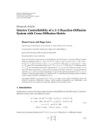
Figure 1. Wired diagrams of (A) a Self-enhancing positive feedback loop, (B) a Self-recovering
positive feedback loop and (C) a negative feedback loop. Solid and dashed arrows represent the
reactions and regulatory effect of components, respectively

2.2.

The mathematical model

Output P is, in general, synthesized proportional to input S and the transcription
factor TF and is degraded in proportion to inhibitor E and X and the output P itself. The
general ODE for P would be
dP
= ks S + ke P − (kd + kr E + kn X) P
(2.1)
dt
Where ks and kd are synthesis and degradation rate constants. The constants ke , kr
and kn represent the effect of TF, E, and X on output P and is referred to as positive
and negative feedback strength. By setting kr = kn = 0, kr = kn = 0, ke = kn = 0 or
ke = kr = 0, we get the equation for output P with ePFL, rPFL and NFL, respectively.
The activation and inhibition of helper TF and inhibitors E and X are governed
by Michaelis-Menten kinetics in order to utilize the nonlinearity[17]. However, any other
reaction types possessing high nonlinearity such as the hill-coefficient equation would do.
The ODE for transcription factor TF, enzyme E and inhibitor X would be
katf P (1 − T F )
kitf T F
dT F

=
−
dt
Jatf + 1 − T F
Jitf + T F

(2.2)

dE
kae (1 − E)
kie P · E
=
−
dt
Jae + 1 − E
Jie + E

(2.3)

dX
=
dt
90

kix X
kax P (1 − X)
−
Jax + 1 − X
Jix + X

1
τ

(2.4)


Flexible controllability of interlocked feedback loops in biological system

The constants of ka and ki are maximal activation and inhibition rates, and those
of Ja and Ji are Michaelis constants (relative to the total concentrations of TF). The
transcription factor TF is more than half of maximum when P > θe = kitf /katf , and
vice versa. The ratio θe = kitf /katf is called the activation level of PFL. The inhibitor
E is more than half of maximum when P > θr = kie /kae , and vice versa. The ratio
θn = kie /kae is called the activation level of PFL.
The constant τ provides a time scale for the activation and inhibition of enzyme E.
The larger τ is, the slower the activation and inhibition of enzyme E is.
The parameter values are listed below: ks = 0.4, kp = 1, kd = 2, kn = 2, katf = 1,
kitf = 0.5, kae = 1, kie = 1, kax = 0.25, kix = 0.1, Jatf = Jitf = 0.01, Jae = Jie = 0.05,
Jax = Jix = 0.005, τ = 1. Changed parameters are specified in the text.

3.

Results

In positive feedback loops, output P somehow promotes its own production. The
output can elevate itself by promoting a helper which in turn elevates the output level or
releases itself from suppression by suppressing its inhibitor.

3.1.

Self-enhancing positive feedback loop: signal amplifier

The typical example of a self-enhancing positive feedback loop is autocatalytic
regulation in which output P promotes its own production by activating activator TF,
Figure 2A
As shown in Figure 2B, the input-output response curves with different feedback
strength are shown. As long as input S increases, product P will increase monotonically.
When output P reaches the activation level of ePFL, P > re , it is able to turn on its
helper, the TF. However, if there is no feedback strength, ke = 0, there is no help from TF
to affect the rate of output P , thus PFL would continue to monotonically increase with
input S, shown as a black, dashed-dotted line. By increasing feedback strength ke , the
transcription factor TF in turn enhances the synthesis rate of product P .
If feedback strength is weak, the enhancement of synthesis rate is small and thus
output P monotonically increases and is enhanced due to simple regulation (red line).
At stronger feedback strength, enhancement of the synthesis rate is larger and
thus output P discontinuously increases, creating bistability or hysteresis (blue line).
Bistability means that output P could be in an either low of high stable steady state (solid
lines) at one input S. Those stable steady states are separated by an unstable steady state,
represented by a dashed line. Output P abruptly changes from one stable state to other one
at two critical values, eSN1 and eSN2, called saddle node bifurcation. The region bound
by SNs, eSN2 < S < eSN1 is called a bistable region.
If feedback strength gets too strong, enhancement of the synthesis rate is strong thus
making the bistability become irreversible bistability (magenta line). That means that once
output P is enhanced, it never goes down even when input S is washed out, S = 0.
91


Nguyen Cuong, Hoang Do Thanh Tung, Trinh Thi Xuan

The summarization is shown in Figure 2C, in which the phase diagram of input S

and feedback strength ke is plotted. The two saddle node bifurcations, eSN1 and eSN2,
occur at smaller input S with stronger feedback strength. When feedback strength is
smaller than a critical value (cusp point), ke < kec , there will be no bistable region with
any input S. And the bistable region becomes irreversible when the feedback strength is
larger than the critical value kei , ke > kei , when eSN2 goes to a negative part of input S.
This ePFL is referred to as an amplification module. Input signal S is passed
through and amplified. The amount of amplification is proportional to the strength
of transcription factor TF, ke TF. The stronger the feedback strength is, the larger the
amplification is.

Figure 2. Self-enhancing and Self-recovering positive feedback loop (ePFL)
(A, C) Input-response curve of ePFL and rPFL with none (dashed-dotted), weak (red), strong
(blue) and very strong (magenta) feedback strength, respectively: The solid and dashed black
lines represent stable and unstable steady state of output P where eSN1 and eSN2 are saddle
node bifurcation of ePFL. (B, D) The Input-feedback strength phase diagrams show regions of
monostability and bistability.

3.2.

Self-recovering Positive feedback loop: signal buffer

Typical examples of a self-recovering positive feedback loop are mutual inhibition
and double negative feedback loops, in which output P removes its suppression by
inhibiting suppressor enzyme E, Figure 2D.
In this case, output P is synthesized proportional to input S. The degradation
rate is proportional to output P and the effect of suppressor E, (kd + kr E)P , where
92


Flexible controllability of interlocked feedback loops in biological system

kd is degradation rate, kr represents the effect of enzyme E on the degradation rate,
the so-called feedback strength. Note that transcription factor E is suppressed when
P > rr = kar /kir , and vice versa. See Figure 2E. The ratio rr = kar /kir is called
the deactivation level of rPFL.
The input-output response curves with different feedback strength kr are shown
in Figure 2E. As long as input S increases, product P is initially suppressed due to the
suppression of enzyme E, which is proportional to feedback strength kr . If there is no
feedback strength, kr = 0, there is no suppression and thus output P monotonically
increases as that of simple regulation, shown as a dashed-dotted line. With the presence of
feedback strength, the output increases but is suppressed. When output is strong enough
to remove its suppression, P > rr , the enzyme is removed and the output is released. If
feedback strength is weak, the suppression on P is small and the recovery is continuous,
shown as a red line. Output P would be discontinuously and abruptly recurred (bistability)
due to the simple regulation once the feedback is stronger, shown as a blue line.
Obviously, feedback strength represents the suppression of P from its inhibitor. The
output is more suppressed with stronger feedback strength and therefore more input S is
needed to produce output P . The ratio rr = kar /kir determines when the inhibitor is
removed.
A summarization is shown in Figure 2F, in which the phase diagram of input S and
feedback strength kr is plotted. As long as feedback strength increases, it is hard to remove
the suppression on inhibiting enzyme E and thus more input S is needed to remove E. The
two saddle node bifurcations move to a larger input S. Note that when feedback strength
is smaller than the critical value (cusp point), kr < krc , there will be no bistable region
with any input S.
This ePFL works as a buffer. When the input signal increases, the output response is
increased but buffered in an inactive state until it overrides its suppressor. Thus, the output
response is delayed from input S. The delay strongly depends on suppressor capacity
(feedback strength) kr . The stronger the suppressor is, the more output is delayed by P.

3.3.

The interlocking of two positive feedback loops: monostability,
bistability, and tristability

The interlocking of two positive feedback loops which show monostability and
bistability would generate monostability, bistability and multistability.
Obviously, each positive feedback loop has two important control parameters feedback strength and the activation level. Feedback strength determines how much the
output is enhanced (ke in ePFL) or suppressed (kr in rPFL). The activation levels, re and
rr , determine the working region of ePFL and rPFL with level of output P , respectively.
Therefore, there are two possibilities that the feedback loop in ePFL and rPFL will be
activated far from each other, (i) re < rr or (ii) re > rr , or (iii) the feedback loop in ePFL
and rPFL can be cooperatively activated, re ≈ rr ,
93


Nguyen Cuong, Hoang Do Thanh Tung, Trinh Thi Xuan

(i) First, consider the case that the ePFL activate at a smaller range of output P than
that in rPFL, re < rr . (See Figure 3A1-Figure 3A4) Output P in iPFL (shown in black)
is initially suppressed from simple regulation (shown as a dashed-dotted line) under the
effect of inhibiting enzyme E, thus output P in iPFL initially follows that of rPFL (shown
in blue). When output P in iPFL reaches the activation level of ePFL, P > re , the TF turns
on to enhance output P . The output P in iPFL continues to increase due to the activation
level of rPFL, P > rr , at which time the inhibiting enzyme E is removed to release
output P . Therefore, there are two transitions of output P corresponding to the different
working region of ePFL and rPFL. The transition might be continuous (monostability)
or discontinuous (bistability) depending on the feedback strength. Both transitions are
continuous when feedback strengths ke and kr are weak (See Figure 3A1) One of them
will be weak and the other will be strong and cause a continuous and a discontinuous

transition. (See Figure 3A2,3) If feedback strengths ke and kr are strong, there will be two
discontinuous transitions. (See Figure 3A4) The two discontinuous transitions might or
might not overlap. Once they overlap, mutltistability emerges. Mutltistability implies that
at one input S there are more than two stable steady states separated by two unstable steady
states. Here, three stable steady states, a low, middle and high level of P , are separated by
two unstable steady states.
(ii) Consider the case that the ePFL activate at a larger range of output P than in
rPFL, re > rm . (See Figure 3C1-Figure 3C4) This means that as long as output P in
iPFL (shown in black) increases and reaches an activation level of rPFL, P > rm , the
inhibiting enzyme E is removed and output P reaccurs as simple regulation (shown as a
black, dashed-dotted line). Output P in iPFL keep increasing until it reaches the activation
level of ePFL, P > re „ and the TF turns on to enhance output P from simple regulation.
Therefore, there are two transitions of output P with corresponding to different working
region of ePFL and rPFL. Depending the feedback strengths ke and kr , the input-output
response of P might have two continuous transitions (See Figure 3C1), a continuous and a
discontinuous transitions (See Figure 3C2,3), or two discontinuous transitions (See Figure
3C4). Here we show a case where the two discontinuous transitions do not overlap and
there is thus no mutltistability. However, mutltistability could be obtained easily by tuning
the activation level or feedback strength.
(iii) When the ePFL and rPFL activate at the same range of output P , re ≈ rm ,
activation of ePFL causes activation of rPFL, and vice versa. Thus they might cooperate
with each other. An interlocking of two PFLs with weak feedback strengths which show
monostability could generate bistability (See Figure 3B1)
With an interlocking of two PFL with weak feedback strength and strong feedback
strength, the bistable region of iPFL is moved and extended from that of a single PFL. For
instance, as seen in Figure 3B2, the bistable region of rPFL is moved and extended to the
left under the effect of ePFL. And the bistable region of ePFL is moved and extended to
the right under the effect of rPFL (See Figure 3B3)
An interlocking of two PFL with strong feedback strengths in the bistable region
94

Flexible controllability of interlocked feedback loops in biological system

of iPFL is extended in both the left and right directions from that of a single PFL. (See
Figure 3C4)

Figure 3. (A1-A4, B1-B4, C1-C4) input-output response of output P at different
activation levels of ePFL and rPFL with different feedback strengths as shown
Red, blue and black lines represent the input-output response of a single ePFL, rPFL and the
interlocking of ePFL and rPFL (iPFL). The dashed-dotted line represents the input-output response
curve of simple regulation. For ePFL feedback strength, ke = 0.3 is weak and 1 is strong. For
rPFL feedback strength kr = 0.5 is weak while 1.5 is strong. For the A’s: re = 0.5, rr = 0.8;
B ′ s : re = rr = 0.5; C ′ s : re = 1, rr = 0.5.

3.4.

The interlocking of a positive and a negative feedback loop:
Relaxation oscillation with flexible controllability of amplitude and
frequency

Oscillation comes from the cooperation of positive and negative feedback loops.
The negative feedback loop drives output P back and forth between low and high steady
states which are from a positive feedback loop. (See Figure 4A) Therefore, oscillation
properties such as amplitude and frequency strongly depend on the feedback strengths of
and the embedded time delay in feedback loops.
Indeed, a too weak or too strong positive feedback strength pushes the system
toward a stable fixed point. In Figure 4C, D increases feedback strength kp and elevates
the right branch of a reverted-N shape null-cline of output P (solid line) causing the
oscillatory system to move toward the stable steady state. If the positive feedback strength

95


Nguyen Cuong, Hoang Do Thanh Tung, Trinh Thi Xuan

is too low, the iPNFL turns out to be a single NFL and thus the iPNFL oscillation will
be shut down. The bifurcation diagram in Figure 6A shows that with either a too weak
(ke < ke1 ) or a too strong (ke2 < ke ) positive feedback strength, the relaxation oscillation
(shown as a blue line) is shutdown. For (ke1 < ke < ke2 ), the iPNFL generates sustained
oscillation with finite amplitude and frequency which are simultaneously varied as long
as positive feedback strength ke changes.

Figure 4. (A, B) Cooperation of PFL and NFL generates relaxation oscillation. (C, D)
Dominant positive feedback strength leads to stable steady state. (E, F) Dominant negative
feedback strength leads to damped oscillation. (G, H) Balanced positive and negative feedback
strengths maintain and enlarge amplitude of sustained oscillation.

A too weak or too strong negative feedback strength will also shut down iPNFL
oscillation. In Figure 4E-F, a negative feedback loop with overwhelming negative
feedback strength kn strongly suppresses output P and the reversed N-shape is
compressed, resulting in a damping of oscillation of output P (shown as a blue solid line).
If the negative feedback strength is too weak, the iPNFL turns out to be a single PFL with
stable steady states rather than one which is oscillatory. The bifurcation diagram in Figure
96


Flexible controllability of interlocked feedback loops in biological system

6B shows that with either a too weak (kn < kn1 ) or too strong (kn2 < kn ) negative
feedback strength, the iPNFL oscillation (blue line) is shutdown. For (kn1 < kn < kn2), ,

the iPNFL generates sustained oscillation with finite amplitude and frequency which are
simultaneously varied as long as negative feedback strength kn changes.
It is shown that increasing positive feedback strength will increase the amplitude
of iPNFL oscillation but reduce the frequency. (See Figure 6A) In contrast, increasing
the negative feedback strength will decrease the amplitude of iPNFL oscillation but
increase the frequency (Figure 6B). In both cases, the oscillation would vanish when
positive or negative feedback strength is overwhelmed. The contradiction of increment
and decrement of amplitude and frequency with respect to single feedback strengths
suggest that changing one feedback strength would unbalance the positive and negative
feedback effects.
To enlarge the amplitude, the positive and negative feedback strengths can be
increased but they must be in agreement with each other in order to maintain the balance
of positive and negative feedback effect. Indeed, by simultaneously increasing positive
and negative feedback strength and keeping the agreement between them, the amplitude
of iPNFL oscillation (shown as a blue orbit) can be enlarged significantly. (See Figure
4G,H) Moreover, the amplitude of iPNFL oscillation (shown as a blue line, in the middle
panel) could be extended as large as we want by maintaining an increase and balance
in positive and negative feedback strength. (See Figure 6C) More importantly, in doing
that, the amplitude of iPNFL oscillation ccan then be controlled freely, independent of the
frequency of iPNFL oscillation (shown as a blue line in the bottom panel) which is almost
the same.

3.5.

The frequency of iPNFL oscillation could be controlled freely and
independently from amplitude by using a time delay

The time delay embedded in the negative feedback which provides time lag
τ0 between output P and its inhibitor X (Figure 5B) might influence the oscillation
frequency. Once might expect that increasing time delay τ would increase time lag τ0

between P and X causing a larger period (at smaller frequency). Indeed, changing time
delay τ does not alter the nullcline structures of the system (See Figure 5A and C) but does
alter time lag τ0 between P and X (Figure 5 and D). The oscillation period is elongated
but the amplitude is not heightened.
The bifurcation diagram of output P with respect to time delay τ shows such
behavior. (See Figure 6D) By varying time delay τ , the frequency of the relaxation
oscillation (shown as a blue line in the bottom panel) could be varied in a broad range.
More importantly, the variation in amplitude of iPNFL oscillation is very small in
comparison to the variation range of time delay τ .

97


Nguyen Cuong, Hoang Do Thanh Tung, Trinh Thi Xuan

Figure 5. Time delay strengthen time lag between output P and its inhibitor X

The smaller time delay (A, B) causes shorter period than the larger time delay (C, D).
Changed parameters: (A, B)τ = 1.0; (C, D)τ = 2.0.

Figure 6.
Figure 6. Bifurcation diagram (top row) with amplitude (middle row) and frequency
(bottom row) of output P with respect to (A) positive feedback strength, (B) negative
feedback strength, (C) lumped feedback strength k(ke = k, kn = ε · k, where ε = kn /ke )
98


Flexible controllability of interlocked feedback loops in biological system

and (D) time delay τ . Black solid and dashed thin lines represent stable and unstable

steady states. Black thick lines represent maxima and minima of oscillation, amplitude and
frequency of dNFL oscillation. Blue (and red) thick lines represent maxima and minima
of oscillation, amplitude and frequency of stable/unstable iPNFL oscillation.

4.
4.1.

Discussion
Multi-stability vs. cell cycle checkpoints

By interlocking two positive feedback loop, the bistability (all-or-none response) is
easier to be generated, as shown Figure 3B1, and while single PFLs could not generate
bistability, iPFLs do. And, bistability is strongly reinforced as shown in Figure 3B2, B3,
and B4, and the bistable regions of the iPFL is strengthened in comparison with that of
a single PFL. More than that, the iPFL can generate tri-stability, a new feature, in which
case the system could be in one of three stable states at the same time. This interlocking
of positive feedback loops is observed at checkpoints in many biological processes,
some examples being G1/S transition, G2/M transition, and morphogenesis in Budding
yeast cell cycle[18, 19] , G2/M of Fission yeast cell cycle[3], G2/M of Mammalian cell
cycle [20], Mitotic trigger of Xenopus Frog Egg [21], EGF receptor signaling[22], B.
subtilis (competence event) [23] and Th1 and Th2 differentiation [24]. This observation
implies that iPFL plays an important role in controlling biological processes. Indeed,
multi-stability is observed and plays a crucial role as a checkpoint in the cell cycle process
[3, 25]. Tyson et. al. has shown that at small size, the activity of cdc2-cdc13 (a complex
that drives the cell cycle) is in the tri-stability region and the first G1 phase corresponds
to the lowest stable state [25].

4.2.

Amplitude and frequency controllability vs. cell cycle mutations

A typical module that governs the mitotic phase of a cell cycle is composed of a PFL
interlocking with an delayed NFL [3, 4, 21, 26, 27]. This setup provides controllability of
amplitude and frequency. By carefully comparing simulation data and experimental data
of many mutations, Chen et. al. has shown that varying the amplitude and frequency
is very crucial for the cell cycle [26]. For example, by reducing the negative feedback
strength of cdh1 (inhibitor X) on the mitosis complex Cdc/Clb, Chen et. al. has shown
that the period of the cell cycle becomes much longer [26]. This phenomenon, observed in
Figure 6B, is due to reduced negative feedback strength. Smolen et. al. utilizes time delay
of the negative feedback loop in iPFL to simulate Drosophila and Neurospora circadian
oscillators [28]. It is shown that time delays are essential to generate circadian oscillations
and that period of circadian oscillators is sensitive to time delay [28].
Acknowledgment
This research is supported by CST Grant 12.02 provided to Young Researchers of
Institute of Information Technology, VAST.
99


Nguyen Cuong, Hoang Do Thanh Tung, Trinh Thi Xuan

REFERENCES
[1] Lee, T.I., Rinaldi, N.J., Robert, F., Odom, D.T., Bar-Joseph, Z., Gerber, G.K., Hannett,
N.M., Harbison, C.T., Thompson, C.M., Simon, I., et al., 2002. Transcriptional
regulatory networks in Saccharomyces cerevisiae. Science 298, pp. 799-804.
[2] Ferrell, J.E., Jr., 2002. Self-perpetuating states in signal transduction: positive
feedback, double-negative feedback and bistability. Curr Opin Cell Biol 14, pp.
140-148.
[3] Novak, B., Pataki, Z., Ciliberto, A., and Tyson, J.J., 2001. Mathematical model of the
cell division cycle of fission yeast. Chaos 11, pp. 277-286.
[4] Chen, K.C., Csikasz-Nagy, A., Gyorffy, B., Val, J., Novak, B., and Tyson, J.J., 2000.

Kinetic analysis of a molecular model of the budding yeast cell cycle. Mol Biol Cell
11, pp. 369-391.
[5] Qu, Z., MacLellan, W.R., and Weiss, J.N., 2003. Dynamics of the cell cycle:
checkpoints, sizers, and timers. Biophys J 85, pp. 3600-3611.
[6] Bell-Pedersen, D., Cassone, V.M., Earnest, D.J., Golden, S.S., Hardin, P.E., Thomas,
T.L., and Zoran, M.J., 2005. Circadian rhythms from multiple oscillators: lessons from
diverse organisms. Nat Rev Genet 6, pp. 544-556.
[7] Tyson, J.J., Chen, K.C., and Novak, B., 2003. Sniffers, buzzers, toggles and blinkers:
dynamics of regulatory and signaling pathways in the cell. Curr Opin Cell Biol 15, pp.
221-231.
[8] Ferrell, J.E., Jr., 1996. Tripping the switch fantastic: how a protein kinase cascade can
convert graded inputs into switch-like outputs. Trends Biochem Sci 21, pp. 460-466.
[9] Ferrell, J.E., and Xiong, W., 2001. Bistability in cell signaling: How to make
continuous processes discontinuous, and reversible processes irreversible. Chaos 11,
pp. 227-236.
[10] Smolen, P., Hardin, P.E., Lo, B.S., Baxter, D.A., and Byrne, J.H., 2004. Simulation
of Drosophila circadian oscillations, mutations, and light responses by a model with
VRI, PDP-1, and CLK. Biophys J 86, pp. 2786-2802.
[11] Kholodenko, B.N., 2000. Negative feedback and ultrasensitivity can bring about
oscillations in the mitogen-activated protein kinase cascades. Eur J Biochem 267, pp.
1583-1588.
[12] Goldbeter, A., 1995. A model for circadian oscillations in the Drosophila period
protein (PER). Proc Biol Sci 261, pp. 319-324.
[13] Pomerening, J.R., Kim, S.Y., and Ferrell, J.E., Jr., 2005. Systems-level dissection
of the cell-cycle oscillator: bypassing positive feedback produces damped oscillations.
Cell 122, pp. 565-578.
[14] Venkatesh, K.V., Bhartiya, S., and Ruhela, A., 2004. Multiple feedback loops are key
to a robust dynamic performance of tryptophan regulation in Escherichia coli. FEBS
Lett 563, pp. 234-240.
100

Flexible controllability of interlocked feedback loops in biological system

[15] Kim, J.R., Yoon, Y., and Cho, K.H., 2008. Coupled feedback loops form dynamic
motifs of cellular networks. Biophys J 94, pp. 359-365.
[16] Kim, D., Kwon, Y.K., and Cho, K.H., 2007. Coupled positive and negative feedback
circuits form an essential building block of cellular signaling pathways. Bioessays 29,
pp. 85-90.
[17] Goldbeter, A., 1991. A minimal cascade model for the mitotic oscillator involving
cyclin and cdc2 kinase. Proc Natl Acad Sci U S A 88, pp. 9107-9111.
[18] Chen, K.C., Csikasz-Nagy, A., Gyorffy, B., Val, J., Novak, B., and Tyson, J.J., 2000.
Kinetic analysis of a molecular model of the budding yeast cell cycle. Mol. Biol. Cell.
11, pp. 369-391.
[19] Ciliberto, A., Novak, B., and Tyson, J.J., 2003. Mathematical model of the
morphogenesis checkpoint in budding yeast. J Cell Biol 163, pp. 1243-1254.
[20] Niida, H., and Nakanishi, M., 2006. DNA damage checkpoints in mammals.
Mutagenesis 21, pp. 3-9.
[21] Novak, B., and Tyson, J.J., 1993. Numerical analysis of a comprehensive model of
M-phase control in Xenopus oocyte extracts and intact embryos. J Cell Sci 106 (Pt 4),
pp. 1153-1168.
[22] Reynolds, A.R., Tischer, C., Verveer, P.J., Rocks, O., and Bastiaens, P.I., EGFR
activation coupled to inhibition of tyrosine phosphatases causes lateral signal
propagation. Nat Cell Biol 5, 447-453.
[23] Hoa, T.T., Tortosa, P., Albano, M., and Dubnau, D., 2002. Rok (YkuW) regulates
genetic competence in Bacillus subtilis by directly repressing comK. Mol Microbiol
43, pp. 15-26.
[24] Yates, A., Callard, R., and Stark, J., 2004. Combining cytokine signalling with
T-bet and GATA-3 regulation in Th1 and Th2 differentiation: a model for cellular
decision-making. J Theor Biol 231, pp. 181-196.

[25] Tyson, J.J., Chen, K., and Novak, B., 2001. Network dynamics and cell physiology.
Nat Rev Mol Cell Biol 2, pp. 908-916.
[26] Chen, K.C., Calzone, L., Csikasz-Nagy, A., Cross, F.R., Novak, B., and Tyson, J.J.,
2004. Integrative analysis of cell cycle control in budding yeast. Mol Biol Cell 15, pp.
3841-3862.
[27] Csikasz-Nagy, A., Battogtokh, D., Chen, K.C., Novak, B., and Tyson, J.J., 2006.
Analysis of a generic model of eukaryotic cell-cycle regulation. Biophys J 90, pp.
4361-4379.
[28] Smolen, P., Baxter, D.A., and Byrne, J.H., 2001. Modeling circadian oscillations
with interlocking positive and negative feedback loops. J Neurosci 21, pp. 6644-6656.

101