Solution manual for financial management principles and applications 12th edition titman keown

Solutions Manual for Financial Management Principles and Applications 12th
Edition by Titman

©2014 Pearson Education, Inc.


Chapter 3
Understanding Financial Statements,
Taxes, and Cash Flows
3-1.

To find the net income, we must subtract all relevant expenses from revenues: cost of goods sold,
operating expenses, interest, and taxes. Following the template from Checkpoint 3.1, we find the
following for Sandifer Manufacturing Company:

Sales
Cost of Goods Sold
Gross Profits
Operating Expenses
Depreciation Expenses
($150,000)
Other Operating Expenses ($300,000)
Total Operating Expenses
Operating Income (EBIT)
Interest Expense
Earnings Before Taxes (EBT)
Income Taxes (@35%)
Net Income

$4,500,000
($3,375,000)

$1,125,000

notes
given
given

given
($450,000)
$675,000
$0
$675,000
($236,250)
$438,750

given
(none mentioned)
=($675,000)*(.35)

Sandifer was able to generate $438,750 in net income from its sales of $4.5M. The $438,750 is now
available to pay out to shareholders (dividends), and/or to reinvest in the business (retained
earnings).
3-2.

We just learned (in Problem 3-1) that Sandifer has $438,750 to allocate to dividends and reinvestment.
If it chooses to reinvest $50,000, then it will have ($438,750  $50,000)  $388,750 to pay out as
dividends (a [$388,750/$438,750]  88.6% payout ratio).

3-3.

Marifield Steel Fabrication earned net income of $500,000, then paid out a dividend of $300,000.

This left ($500,000  $300,000)  $200,000 to be retained by the firm to finance growth. 





63

(As noted in the text, firms with taxable income greater than $18.33M, the top of the 7th bracket,
are indifferent between the progressive scheme and a flat rate of 35%.)



64

3-4.

Titman/Keown/Martin

   Twelfth Edition

Barrington Enterprises earned $4M in taxable income. Using the corporate tax rates given in
Section 3.3 of the chapter, we find the following:

bracket
#1
#2
#3
#4
#5

(marginal)
taxable income
$50,000
$25,000
$25,000
$235,000
$3,665,000

cumulative
income taxed
$50,000
$75,000
$100,000
$335,000
$4,000,000

marginal
tax rate
15%
25%
34%
39%
34%

tax liability
$7,500
$6,250
$8,500
$91,650

$1,246,100

cumulative
tax liability
$7,500
$13,750
$22,250
$113,900
$1,360,000

average
tax rate
15.00%
18.33%
22.25%
34.00%
34.00%

Barrington’s total tax liability is $1,360,000, for an average tax rate of ($1,360,000/$4,000,000)  34%.
The chart above is very close to that in Section 3.3. However, we will explain the entries, using the
calculations for bracket #3 (highlighted in the chart) as an example:
Bracket #3 is shown in the text to apply to taxable income between $75,001 through $100,000.
Thus, the bracket applies to $25,000, which is what we have entered in the “(marginal) taxable
income” column. The “cumulative income taxed” column shows $100,000, meaning that when
we have moved through this third bracket, we will have taxed our first $100,000 of taxable income.
Since we move all the way through the third bracket, we generate ($25,000 taxable income in
bracket)  (34% marginal tax rate)  $8500 in tax liability from that bracket. Added to the tax we
owed for the first two brackets, this implies a total liability so far of ($13,750  $8500)  $22,250.
This tax liability is a weighted average of the rates whose brackets we’ve passed through: 15%,
25%, and 34%. This average equals ($22,250 tax liability so far)/($100,000 taxed so far)  22.25%,

a value between 15% and 34%.
Note that the final average tax rate for the firm is 34%. Our average tax rate equals our marginal
rate, even though our first dollars were taxed at 15% and 25%! What’s going on?
The chart below shows how the fourth bracket’s 5% surcharge (to 39%) takes away the benefits of
the first two brackets. Column D shows how each bracket’s taxable income increment would be
taxed, if exposed to a flat rate of 34%. Column E then shows the difference between this hypothetical
flat 34% tax and the actual, progressive rates. The first two brackets save the company $11,750
relative to the flat 34%. However, this is exactly the amount recouped by the 5% surcharge as the
company moves all the way though the fourth bracket. Companies that have more than $335,000 in
taxable income, but less than $10M, are indifferent between the actual progressive system and a flat
rate of 34%.
A
bracket
#1
#2
#3
#4
#5

(marginal)
taxable income
$50,000
$25,000
$25,000
$235,000
$3,665,000

B
cumulative
income taxed

$50,000
$75,000
$100,000
$335,000
$4,000,000

marginal
tax rate
$0
25%
34%
39%
34%

C = A*B
tax liability
$7,500
$6,250
$8,500
$91,650
$1,246,100

D = A*(34% )
cumulative
tax liability
$7,500
$13,750
$22,250
$113,900
$1,360,000

average
tax rate
$0
18.33%
22.25%
34.00%
34.00%

E=D-C

tax liability
$ saved from
at 34%
actual tax rates
$17,000
$9,500
$8,500
$2,250
$8,500
$0
$79,900
($11,750)
$1,246,100
$0
SUM =
$0

(As noted in the text, firms with taxable income greater than $18.33M, the top of the 7th bracket,
are indifferent between the progressive scheme and a flat rate of 35%.)

Solutions to End-of-Chapter Problems—Chapter 3 65

3-5.

Sanderson, Inc.’s situation before the dividends is:

Sales

$3,000,000
($2,000,000)
$1,000,000

Cost of Goods Sold
Gross Profits
Operating Expenses
Depreciation Expenses
($100,000)
Other Operating Expenses ($400,000)
Total Operating Expenses
($500,000)
Operating Income (EBIT)
$500,000
Interest Expense
($150,000)
Earnings Before Taxes (EBT)
$350,000

notes

given
given

given
given
given
given

However, before we can determine the firm’s tax liability, we must consider the tax due on its
dividends received. The firm received $50,000 from a company in which it owned less than 20%.
Because of the dividends-received deduction, Sanderson only needs to pay taxes on (1  0.70)  30%
of these dividends. This will add (30%)  ($50,000)  $15,000 to the firm’s taxable income.
(Dividends paid to the firm’s own shareholders are made after taxes are paid. They therefore will
not affect the firm’s tax liability.)
Thus, we have:

Earnings Before Taxes (EBT)
$350,000
Dividends Received, after 70% Dividends Received Deduction $15,000
Total Taxable Income $365,000
(marginal)
cumulative marginal
cumulative average
bracket taxable income income taxed tax rate tax liability tax liability tax rate
#1
$50,000
$50,000
15%
$7,500
$7,500

15.00%
#2
$25,000
$75,000
25%
$6,250
$13,750
18.33%
#3
$25,000
$100,000
34%
$8,500
$22,250
22.25%
#4
$235,000
$335,000
39%
$91,650
$113,900
34.00%
#5
$30,000
$365,000
34%
$10,200
$124,100
34.00%
Sanderson has $365,000 in taxable income, so it will end up in the 5th tax bracket. Thus, as we saw

in Problem 3-4, this means that Sanderson’s average tax rate equals its marginal rate of 34%.


66

3-6.

Titman/Keown/Martin

   Twelfth Edition

The statement below outlines the situation of the Robbins Corporation:

Sales
Cost of Goods Sold
Gross Profits
Operating Expenses
Depreciation Expenses
Cash Operating Expenses
Total Operating Expenses
Operating Income (EBIT)
Interest Expense
Earnings Before Taxes (EBT)

$1,000,000
($600,000)
$400,000
($50,000)
($100,000)

Earnings Before Taxes (EBT)
Dividends Received, after 75% Dividends Received Deduction
Total Taxable Income

($150,000)
$250,000
($200,000)
$50,000

notes
given
given

given
given
given
given

$50,000
$10,000
$60,000

Because Robbins owns between 20% and 79% of a firm’s shares, the dividend it receives from
that firm are subject to a 75% dividends received deduction. Thus, Robbins is only taxed on
(100%  75%)  25% of its dividends received, or (25%)  ($40,000)  $10,000.
Adding Robbins’ $10,000 in taxable dividends to its $50,000 in taxable income from operations
gives the firm a total of $60,000 in taxable income. We can now compute its tax liability as:
(marginal)
cumulative marginal
cumulative average

bracket taxable income income taxed tax rate tax liability tax liability tax rate
#1
$50,000
$50,000
15%
$7,500
$7,500
15.00%
#2
$10,000
$60,000
25%
$2,500
$10,000
16.67%
Robbins finishes in the middle of the second bracket, so its marginal tax rate (the rate on its next
dollar of income, which will still be in the second bracket) is 25%. Its average tax rate is the weighted
average of the $50,000 taxed in the first bracket at 15%, and the ($60,000  $50,000)  $10,000
taxed at 25% in the second bracket: ($50,000/$60,000)  (15%)  ($10,000/$60,000)  (25%) 
(0.8333)  (15%)  (0.1667)  (25%)  16.67%.
As for additional action: Robbins made $1M in sales, but generated only ($50,000  $10,000 tax
liability)  $40,000 in after-tax (net) income (ignoring the dividends it received). It may want to
search for operating efficiencies to improve its profit margins. Its interest expenses, in particular,
seem high.
Note that we did not consider Robbins’ dividend payments to its own stockholders here, since those
payments are made after taxes are paid.


Solutions to End-of-Chapter Problems—Chapter 3 67

3-7.

For J.P. Hulett, we have the following statement calculating taxable income:

Sales
Cost of Goods Sold
Gross Profits
Operating Expenses
Depreciation Expenses
Other Operating Expenses
Total Operating Expenses
Operating Income (EBIT)
Interest Expense
Earnings Before Taxes (EBT)

$4,000,000
($3,000,000)
$1,000,000
($350,000)
($500,000)

notes
given
given
given
given

($850,000)
$150,000
$0

$150,000

Earnings Before Taxes (EBT)
Dividends Received, after 100% Dividends Reveived Deduction
Total Taxable Income

(none was mentioned)

$150,000
$0
$150,000

Since Hulett owns more than 80% of the shares of the firm from which it received dividends, none
of the dividends are taxable to Hulett, and we can ignore them.
Given Hulett’s taxable income of $150,000, we can find its tax liability as follows:
(marginal)
cumulative marginal
cumulative average
bracket taxable income income taxed tax rate tax liability tax liability tax rate
#1
$50,000
$50,000
15%
$7,500
$7,500
15.00%
#2
$25,000
$75,000
25%

$6,250
$13,750
18.33%
#3
$25,000
$100,000
34%
$8,500
$22,250
22.25%
#4
$50,000
$150,000
39%
$19,500
$41,750
27.83%
Hulett’s taxable income of $150,000 takes it up to the fourth bracket, where its marginal tax rate
(tax on next dollar of income) is 39%. Its average tax rate is a weighted average of the tax rates
from the first through fourth bracket: 15%, 25%, 34%, and 39%. For Hulett, this average is
($41,750/$150,000)  27.83%. (If Hulett had made it all the way through the fourth bracket, its
average tax rate would have been 34%, as we discussed in Problem 3-4.)
3-8.

The statement below shows how we can compute the taxable income for G.R. Edwin, Inc.:

Sales
Cost of Goods Sold
Gross Profits
Operating Expenses

Operating Income (EBIT)
Interest Expense
Earnings Before Taxes (EBT)

$6,000,000
($3,000,000)
$3,000,000
($2,600,000)
$400,000
($30,000)
$370,000

notes
given
given
given
given


68

Titman/Keown/Martin

   Twelfth Edition

Edwin therefore has taxable income of $370,000. Using the corporate tax tables from the chapter,
we can therefore determine the tax liability as:
(marginal)
cumulative marginal
cumulative average

bracket taxable income income taxed tax rate tax liability tax liability tax rate
#1
$50,000
$50,000
15%
$7,500
$7,500
15.00%
#2
$25,000
$75,000
25%
$6,250
$13,750
18.33%
#3
$25,000
$100,000
34%
$8,500
$22,250
22.25%
#4
$235,000
$335,000
39%
$91,650
$113,900
34.00%
#5

$35,000
$370,000
34%
$11,900
$125,800
34.00%
Since the firm’s taxable income moved it beyond the fourth bracket and into the fifth, Edwin’s
average tax rate is 34% ($125,800 tax liability/$370,000 taxable income), as is its marginal tax rate.
Remember that the fourth bracket has a surcharge that gradually takes away the benefits of initially
moving through the 1st (15%) and 2nd (25%) brackets. Moving all the way through the fourth
bracket, as Edwin did, means that all of those low-rate benefits are taken away, and the firm is left
as if it had paid a flat rate of 34% from the beginning.
3-9.

Meyer Inc. has taxable income of $300,000, which is in the fourth tax bracket. Since Meyer won’t
move all the way through this bracket (its upper limit is $335,000, higher than Meyer’s EBT), its
marginal tax rate will be the 4th bracket’s rate, 39%. Also, since Meyer will not have moved all the
way through the 4th bracket, it will not have all of the benefits of the low-rate 1st and 2nd brackets
taken away; its average tax rate will therefore be less than 34%. We can find its tax liability and
average tax rate as follows:
(marginal)
cumulative marginal
cumulative average
bracket taxable income income taxed tax rate tax liability tax liability tax rate
#1
$50,000
$50,000
15%
$7,500
$7,500

15.00%
#2
$25,000
$75,000
25%
$6,250
$13,750
18.33%
#3
$25,000
$100,000
34%
$8,500
$22,250
22.25%
#4
$200,000
$300,000
39%
$78,000
$100,250
33.42%
EBT: given



Meyer pays a total of $100,250 in taxes, on a taxable income of $300,000. Its average tax rate is
 $100,250 
therefore 
  33.42%.

 $300,000 
3-10. Boisjoly Productions has $19M of taxable income. This puts the firm into the very highest tax
bracket, the eighth, in which the marginal tax rate is 35%. In earlier problems (e.g., 3-8), we saw
that firms whose taxable income fell into the 5th bracket had their low-rate brackets’ benefits taken
away, leaving them with a flat 34% tax rate. Firms like Boisjoly that make it all the way into the
8th bracket have a similar but more severe situation: They have all of their low-rate benefits taken
away, leaving them with a flat 35% rate.


Solutions to End-of-Chapter Problems—Chapter 3 69
taxable income = $19,000,000

bracket
#1
#2
#3
#4
#5
#6
#7
#8

A

B

C

(marginal)
taxable income

$50,000
$25,000
$25,000
$235,000
$9,665,000
$5,000,000
$3,333,333
$666,667

cumulative
income taxed
$50,000
$75,000
$100,000
$335,000
$10,000,000
$15,000,000
$18,333,333
$19,000,000

marginal
tax rate
15%
25%
34%
39%
34%
35%
38%
35%

D = A*C

E

F = E/B

tax liability
$7,500
$6,250
$8,500
$91,650
$3,286,100
$1,750,000
$1,266,667
$233,333

cumulative
tax liability
$7,500
$13,750
$22,250
$113,900
$3,400,000
$5,150,000
$6,416,667
$6,650,000

average
tax rate

15.00%
18.33%
22.25%
34.00%
34.00%
34.33%
35.00%
35.00%

How does this happen? We can track the benefits from the lower-rate brackets and the costs of the
higher-rate brackets as shown below:
A
bracket
#1
#2
#3
#4
#5
#6
#7
#8

(marginal)
taxable income
$50,000
$25,000
$25,000
$235,000
$9,665,000
$5,000,000

$3,333,333
$666,667

B
cumulative
income taxed
$50,000
$75,000
$100,000
$335,000
$10,000,000
$15,000,000
$18,333,333
$19,000,000

marginal
tax rate
15%
25%
34%
39%
34%
35%
38%
35%

C = A*B
tax liability
$7,500
$6,250

$8,500
$91,650
$3,286,100
$1,750,000
$1,266,667
$233,333

D = A*(34% )
cumulative
tax liability
$7,500
$13,750
$22,250
$113,900
$3,400,000
$5,150,000
$6,416,667
$6,650,000

average
tax rate
$0
18.33%
22.25%
34.00%
34.00%
34.33%
35.00%
35.00%

E=D-C

tax liability
$ saved from
at 35%
actual tax rates
$17,500
$10,000
$8,750
$2,500
$8,750
$250
$82,250
($9,400)
$3,382,750
$96,650
$1,750,000
$0
$1,166,667
($100,000)
$233,333
$0
SUM =
$0

cumulative
savings
$10,000
$12,500
$12,750

$3,350
$100,000
$100,000
$0
$0

Column D in the chart above calculates the tax liability for a bracket, assuming that the rate for that
bracket is 35%. Column E then compares that hypothetical 35% tax liability with the actual liability
for the bracket. For brackets whose rates are less than 35%, column E therefore shows a savings—a
benefit from paying the actual, lower rate rather than 35%. However, in brackets #4 and #7, column
E is negative. In these brackets, the marginal rates are greater than 35%. These brackets are taking
back the benefits of the lower-rate brackets. If a taxpayer passes all the way through the 7th bracket,
as Boisjoly does, then all of the low-rate benefits are taken away. The taxpayer whose taxable
income is greater than $18.33M pays a flat 35%.
3-11. Caraway Seed’s balance sheet is shown below:

ASSETS
Current Assets
$50,000
Net Fixed Assets $250,000

LIABILITIES
Current Liabilities
Long-Term Debt
TOTAL LIABILITIES

$30,000
$100,000
$130,000

OWNERS' EQUITY
STOCKHOLDERS' EQUITY
$170,000
TOTAL ASSETS

$300,000

TOTAL L & OE

$300,000

(plug)


70

Titman/Keown/Martin

   Twelfth Edition

A. Caraway’s total assets are the sum of its current (short-term) assets of $50,000 and its fixed
(long-term) assets of $250,000: $300,000. Since this is what Caraway has, this is the amount for
that it has received funding. Caraway uses two types of funding: debt and equity. It therefore
must be true that its debt funding received plus its equity funding equals the total, $300,000.
We are told that Caraway has $30,000 in current (short-term) debt, plus $100,000 in long-term
debt. It therefore has received a total of ($30,000  $100,000)  $130,000 in debt funding. Since
it has $300,000 in assets, it must be that ($300,000  $130,000)  $170,000 in funding has come
from equity. (Once we know total assets and total liabilities, then, total equity is just a plug figure.)
B. If we focus on current assets and liabilities, we can find net working capital, which is defined in
equation 3-5 as:

net working capital = current assets  current liabilities
= $50,000  $30,000  $20,000.
This is the amount of liquid assets that Caraway has, above and beyond what it needs to make
payments over the next year. Given that its current liabilities are $30,000, a cushion of $20,000
seems to imply that Caraway is very liquid.
C. Knowing that the firm’s $30,000 in current liabilities is comprised of $20,000 in accounts
payable and $10,000 in notes payable does not affect working capital, which is based on total
current liabilities and assets. (See Figure 3.1, where working capital is defined graphically;
current liabilities there include A/P and N/P.)
3-12. First, let’s categorize the accounts we were given:

Note that expenses and revenues go on the income statement, while assets, liabilities, and equity go
on the balance sheet.
As shown on the next page, we will find retained earnings as the plug figure that will equate total
assets with total liabilities and owners’ equity. We use the following 2-step process:
STEP 1
total assets =
less total liabilities =
total equity =

STEP 2
$120,650
($60,400)
$60,250

total equity =
less common stock =
retained earnings =

$60,250

($45,000)
$15,250


Solutions to End-of-Chapter Problems—Chapter 3 71

Now that we know which accounts belong to which statement, we can create the statements as follows:

BELMOND, INC.
INCOME STATEMENT (for year ended mm/dd/yy)
Sales
Cost of Goods Sold
Gross Profits
Operating Expenses
Depreciation Expenses
Operating Expenses
General and Administrative Expenses
Total Operating Expenses
Operating Income (EBIT)
Interest Expense
Earnings Before Taxes (EBT)
Taxes
Net Income

$12,800
($5,750)
$7,050
($500)
($1,350)
($850)

($2,700)
$4,350
($900)
$3,450
($1,440)
$2,010

BELMOND, INC.
BALANCE SHEET (as of mm/dd/yy)
ASSETS
Current Assets
Cash
Accounts Receivable
Inventory
Total Current Assets
Buildings & Equipment
Less: Accumulated Depreciation
Total Fixed Assets

TOTAL ASSETS

$16,550
$9,600
$6,500
$32,650
$122,000
($34,000)
$88,000

$120,650

LIABILITIES
Current Liabilities
Accounts Payable
Short-term Notes Payable
Total Current Liabilities

$4,800
$600
$5,400

Long-Term Debt
Total Liabilities

$55,000
$60,400

OWNERS' EQUITY
Common Stock
Retained Earnings
Total Common Stockholders' Equity
TOTAL L & OE

$45,000
$15,250
$60,250
$120,650

(plug)

Now that we’ve identified Belmond’s current assets and current liabilities, we can find the firm’s
net working capital as the difference between them:
current assets
 $32,650
current liabilities  ($5,400)
net working capital  $27,250


72

Titman/Keown/Martin

   Twelfth Edition

If I were asked to assess Belmond’s financial position, I’d say:
 It has adequate liquidity, given that its current assets are $32,650 while current liabilities are
only $5,400—resulting in a strong net working capital position of $27,250.
 It is managing its costs well: COGS is only 45% of sales; operating expenses are 21%; interest
expenses are 7%; net income is almost 16%.
 Its retained earnings seem relatively low, which is odd, given the rest of the results.
 Its cash seems extremely high, given its sales (annual sales < cash!).
Overall, Belmond seems to be well managed and in good financial shape.
3-13. We first classify Warner’s accounts as follows:

Expenses and revenues belong on the income statement; assets, debt, and equity belong on the balance
sheet. Note that accrued expenses are a current liability—this represents an accumulation of expenses
taken on the periodic income statements, and are the amount the firm must pay (thus, a liability).
(The same applies to taxes payable.)
Given these assignments, we can create the firm’s balance sheet and income statement as shown on
the next page.

ASSETS
Current Assets
Cash
Accounts Receivable
Inventory
Total Current Assets
Buildings & Equipment
Less: Accumulated Depreciation
Total Fixed Assets

$225,000
$167,500
$99,300
$491,800
$895,000
($263,000)
$632,000

TOTAL ASSETS $1,123,800

LIABILITIES
Current Liabilities
Accounts Payable
Accrued Expenses
Taxes Payable
Notes Payable
Total Current Liabilities

$102,000
$7,900

$53,000
$75,000
$237,900

Long-Term Debt
Total Liabilities

$334,000
$571,900

OWNERS' EQUITY
Common Stock $289,000
Retained Earnings $262,900
Total Common Stockholders' Equity $551,900
TOTAL L & OE $1,123,800


Solutions to End-of-Chapter Problems—Chapter 3 73

Warner’s financials reveal no glaring, severe problems. The firm seems to be doing well managing
its expenses. Its COGS is about 52% of sales; operating expenses are 25%; net income is 13%. It is
adequately liquid: Its net working capital is $253,900 (current assets of $491,800 are over 2  current
liabilities of $237,900). In fact, the firm may be too liquid: Cash is 20% of total assets, which seems
high, especially since  of the current liabilities total just over 21%. The firm is running lean on
inventory (9% of assets), which is positive. Long-term debt is only 30% of assets; interest expense
is less than 1% of sales. (Given that the firm’s tax bill was almost 9% of sales, it could probably
benefit from more leverage.)
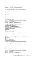
3-14. The values from Goggle’s cash flow statement are graphed below:

$5,000

$3,000

$1,000
cash from operating activities

2007

2008

2009

cash from investing activities

2010
($1,000)

($3,000)

($5,000)

($7,000)

cash from financing activities
net change in cash


74

Titman/Keown/Martin

   Twelfth Edition

A. The black dashed curve is the net change in cash. In 2007 and 2009, this goes slightly negative.
However, this is not from operations: The blue curve shows cash from operating activities,
which is increasing steadily throughout the period.
B. Instead, the net cash is negative because Goggle has been investing heavily in capital assets,
especially in 2009 (see the red curve). In fact, over the last four years, Goggle has invested
$15,900 in capex (this is just the sum of net “cash from investing activities”).
C. Looking at the green curve, we can track Goggle’s activities in the financial markets. The firm
has issued stock in each of the four years (sum of stock issuance  $8024). This alone was
insufficient to pay for its capex, but nonetheless was a major source of funds. They have issued
no new debt; in fact, they have retired small amounts of debt over the last two years (total of $7)
and have earned $1005 in interest cash flow. (The rest of the cash for the capital assets therefore
came from operations.)
D. Thus over the last four years, Goggle’s management has spent heavily on new capital assets,
financing those purchases with operating cash flow plus significant inflows from stock sales.
The largest of these stock sales occurred in 2008, with issuance of $4400. This has tapered off
to only $24 in the most recent year; however, as their operating cash flows have ramped up to
$5600 in 2010, exceeding their capital investment (although its capital expenditures were still
fairly strong in 2010, at $3600).
The firm has paid no dividends over the period, which has preserved cash for capital investment.
The firm appears to be in the “growth” phase of its lifecycle: high capex, low dividends.
The firm has had increasing cash flow from operations: Net income, depreciation, and working
capital changes have all contributed positively. (We should not be surprised by the depreciation,
at least given the heavy investment in new assets.) The net income growth is very positive, as is
the ability of the firm to decrease its working capital investment.
Goggle has also received interest inflows over the last two years, which, at $400 and $600, were
noticeable contributors to the firm’s cash flows.
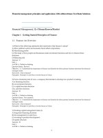
3-15. BigBox’s cash flows are graphed below:

$18,800

$13,800

$8,800

$3,800

cash from operating activities
cash from investing activities
cash from financing activities
net change in cash

2007

2008

2009

2010

($1,200)

($6,200)

($11,200)

($16,200)

Solutions to End-of-Chapter Problems—Chapter 3 75

A. BigBox has generated positive cash flows from operations, as shown by the blue curve. However,
this growth has slowed significantly lately, with 2010’s operating cash flows being almost
indistinguishable from 2009’s.
B. The company has made significant capital investments over each of the four years, increasing
the amount every year. The total over the full period is $56,800.
C. These investments have not been financed with net new issuance in the financial markets, since
cash from financing activities has been negative in each of the four years. (Capex therefore
came from operating cash flow, the only significant source of cash the firm has.) The firm has
paid a large dividend each year (with a four-year total of $11,100), and has also retired stock
each year. There have been some financing cash inflows from debt issuance—the firm has
issued debt in every year except 2009, when a nominal amount ($100) was retired (issuance in
the other three years totaled $9600, almost sufficient to pay the firm’s dividends). The firm is
therefore substituting debt for equity.
Thus it appears that over the last four years, the firm has:
 Generated steady growth in net income, and some growth in depreciation cash flow
 Received positive cash flow from reductions in working capital investments
 Made significant and growing expenditures on capital assets (of between 123% and 127% of net
income each year)
 Paid steadily growing dividends (of between 22% and 28% of net income)
 Retired stock each year, with the largest retirement in the most recent year, while issuing debt
(although the debt amounts issued were always less than the stock amounts retired)
Since the firm’s operating cash flows were insufficient in 2010 to support its aggressive capex and
stock retirements, its net change in cash was significantly negative for this year.
This firm, unlike Goggle in Problem 3-14, appears to be in its mature phase, despite its capital
expenditures. Rather than the rapid growth of a young firm, this firm is closer to a mature, steady
state.
3-16. The first part of the question regarding the quality of earnings ratio appears to be for a different year

than presented in the table provided for parts a) and b). Using the information provided in
introductory portion of the question we then calculate as follows:
Quality of earnings ratio = cash flow from operations / net income
= $575,000 / $750,000 = .7667 = 76.67%
Without further detail, as given in the Boswell example of the text, we can only say that the firm
depended on about 77% of its cash flow from its operating income stream and about 23% from nonoperating sources.
a) Part a) only details information that is used to answer Part b).
b) In order to calculate the average capital acquisitions ratio for Kabutell, we can use the adapted
form of equation 3-9 that was used in the Boswell example on page 64 of the text.
Capital acquisitions ratio =
3-yr avg cash flow from operations / 3-yr avg cash paid for CAPEX =
{($478 + $403 + $470) / 3 } / {($459 + $447 + $456) / 3} = 0.9919 = 99.19%
This means that for the last 3 years, Kabutell was able to finance 99.19% of its capital
expenditures with operating cash flow.


76

Titman/Keown/Martin

   Twelfth Edition

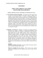
3-17. Using the link to Yahoo Finance the following statement of cash flows
were found for Home Depot and Lowes:


Solutions to End-of-Chapter Problems—Chapter 3 77


78

Titman/Keown/Martin

   Twelfth Edition

2013

2012

2011

4,535,000

3,883,000

3,338,000

6,975,000
1,312,000

6,651,000
1,221,000

4,585,000
1,096,000

Quality of Earnings Ratio =
CF from Oper / Net
Income

153.80%

171.29%

137.36%

Capital Acquisitions Ratio =
CF From Oper / Cash Paid
for CAPEX

531.63%

544.72%

418.34%

2013

2012

2011

1,959,000

1,839,000

2,010,000

3,762,000
1,211,000

4,349,000
1,829,000

3,852,000
1,329,000

Quality of Earnings Ratio =
CF from Oper / Net
Income

192.04%

236.49%

191.64%

Capital Acquisitions Ratio =
CF From Oper / Cash Paid
for CAPEX

310.65%

237.78%

289.84%

Home Depot
Net Income
CF from Operating

Activities
CAPEX

Lowes
Net Income
CF from Operating
Activities
CAPEX

a) As calculated above, the quality of earnings ratio for both Home Depot and Lowes is high and
above 100%. For Home Depot, the values are 153.80%, 171.29%, and 137.26%, respectively.
For Lowes the values are 192.04%, 236.49%, and 191.64%, respectively. These numbers
suggest that the quality of earnings for both firms is very high.
b) Home Depot has a much larger amount for an adjustment to net income as well as a positive
and large adjustment to operating activities. While either of those adjustments may be
innocuous, a serious investor would need to understand both of the items.


Solutions to End-of-Chapter Problems—Chapter 3 79

c) As calculated above, the quality of earnings ratio for both Home Depot and Lowes is high and
above 100%. For Home Depot, the values are 531.63%, 544.72%, and 418.34%, respectively.
For Lowes the values are 310.65%, 237.78%, and 289.84%, respectively.
d) Home Depot is able to cover its CAPEX through its cash flow a greater number of times, but
both firms have the means to expand their CAPEX significantly. Lowe’s appears to have issued
debt in 2013 and would therefore have been more active in the capital markets than Home
Depot.