Brownian Motion
Bạn đang xem bản rút gọn của tài liệu. Xem và tải ngay bản đầy đủ của tài liệu tại đây (564.55 KB, 16 trang )
21
Brownian Motion
It was shown at the end of the last chapter that in the limit of an infinite number of infinitesimally
small steps, the behavior of a discrete time martingale converges to a Brownian motion. This
chapter undertakes a review of the properties of Brownian motion. The story of buffeted pollen
grains is very familiar by now and the busy reader is probably anxious to move on to the
pricing of financial instruments as quickly as possible. However, there are important insights
to be gained by considering physical displacements rather than stock price movements. In this
chapter we lean rather heavily on such insights, so the description is couched in terms of the
movement of a particle in one dimension. We can then exploit physical concepts such as total
distance traveled in a certain time, which have no meaning if we consider only stock price
movements.
21.1 BASIC PROPERTIES
(i) The use of the expressions normally distributed, Gaussian distribution, Wiener process and
Brownian motion has been rather casual in previous parts of this book, as indeed in most of
the options literature and in practice. The following points should clarify the position:
r
Normal distribution refers to the distribution of a single random variable. It is of course
possible for two normally distributed variables to be correlated, in which case they enjoy a
bivariate normal distribution. A process cannot be said to be normally distributed.
r
However, if each of the random variables in a process H
0
,..., H
j
are normally distributed,
the process is called Gaussian.
r
A Brownian motion is the continuous Gaussian process which is described in the next
paragraph.
r
A Wiener process is defined as a continuous adapted martingale whose variance is equal to
the time over which the variance is measured. It can be proved that a Wiener process must
be a Brownian motion (Levy’s theorem).
(ii) A continuous random process W
t
is a standard Brownian motion if it has the following
properties:
(A) It is a martingale starting at W
0
= 0.
(B) It is continuous, i.e. no jumps.
(C) It is a Markov process: the distribution of W
t
− W
s
depends only on the value of W
s
and
not on any previous values.
(D) W
t
− W
s
is normally distributed with mean 0 and variance (t − s).
Any Brownian motion can of course be constructed from a standard Brownian motion merely
by applying a scaling factor for the volatility and resetting the starting point.
(iii) In terms of physical movement, a Brownian particle moves continuously along a line after
starting at the point zero. At time t its position is given by W
t
. Intuition suggests that at time
21 Brownian Motion
t + δt its position can be expressed as W
t
+ δW
t
. However, δW
t
is a random variable with
mean zero, which means that at each instant it has an equal chance of being positive or negative
and has an unpredictable size. The function W
t
is therefore not differentiable at any point. A
quick glance at Figure 21.1 confirms this property; it is clear just from the form of the graphs
that the first derivative with respect to time is undefined, while the second derivative is infinite,
i.e. the function is completely “spiky” at all points.
As an aside, it is interesting to note that although Brownian motion originally referred to a
physical phenomenon, the mathematical process defined in this section could never apply to
a physical process. The infinite spikiness means that an infinite amount of energy would be
needed to get a particle with non-zero mass to follow a Brownian path.
(iv) Figure 21.1 shows a path following a standard Brownian motion. The first graph shows a par-
ticular path from time 0 to time 1 year. Suppose we now want to see what is going on in greater
detail. We take the part of the year within the dotted box and double it in size, expanding both
the x- and y-axes by a factor of two; this is shown in the second graph. Suppose we again want
to examine the path in greater detail. We double half of the second path to give the third graph.
Although the specific paths in the first and third graphs are not identical, they nonetheless
have the same general appearance in that they have the same degree of “jaggedness”, i.e. they
have the same apparent variance. The reason for this is straightforward: the variance of a
Brownian motion is proportional to the time elapsed. Thus, expanding both the x-axis (which
represents time) and the y-axis (which illustrates variance) by the same factor will result in
paths of similar appearance, despite the fact that the scales of the graph have changed. In a
word, Brownian motion is fractal: however many times we select a subsection of a path and
magnify it, its variance looks the same. Obviously, the scale of the x- and y-axes changes as
we do this, so that the actual variance of the section of the path chosen is always proportional
to the time period over which it is measured. So what, you might say: well, it does have some
unexpected consequences.
-1.6
-1.2
-0.8
-0.4
0
0.4
0.8
1.2
1.6
0
years
1
-0.8
-0.4
0
0.4
0.8
.25
.75
years
-0.4
0
0.4
.375
.625
years
Figure 21.1 Fractal nature of Brownian motion
Most people looking at graphs like those in Figure 21.1, would feel intuitively that if the
graphs were continued to the right far enough, the Brownian path would cross the zero line
quite often. If the x -axis were extended to be a billion times longer, the path would cross
the zero line very, very often. In fact, it is reasonable to assume that if the length of the time
axis increases to ∞, then the path will be observed to cross the zero line infinitely often.
Consider a standard Brownian motion at its starting point W
0
= 0. We take a snapshot of
the beginning of the path and blow it up a billion times. Surprise, surprise: having the fractal
property described above, it “looks” just like the original path, although when we look at the
scales of the x- and y-axes, they only cover tiny changes in time and value. But we have already
admitted that we believe that if we extended the x-axis a billion times, the Brownian path will
244
21.2 FIRST AND SECOND VARIATION OF ANALYTICAL FUNCTIONS
cross the zero line a very large number of times. We must therefore concede that given the
fractal property of the path, it will cross the zero line a very large number of times in the tiny
time interval at its beginning. The same must of course hold true any time a Brownian motion
crosses the zero line.
Indeed, it can be proved quite rigorously that when a Brownian path touches any given
value, it immediately hits the same value infinitely often before drifting away. Eventually, it
drifts back and hits the same value infinitely often again – and then it repeats the trick an
infinite number of times! These thought games are fun, but might not seem to have much to do
with option theory. However, this property of Brownian motion, known as the infinite crossing
property, is central to the pricing of options. It will be shown in Chapter 25 that without it,
options would be priced at zero volatility.
21.2 FIRST AND SECOND VARIATION
OF ANALYTICAL FUNCTIONS
The object of the following chapters is to develop some form of calculus or set of computational
procedures which can adequately describe functions of a Brownian motion, W
t
. We really have
no right to expect to find such a calculus; after all, classical (Riemann) calculus was evolved
with well-behaved, continuous, differentiable functions in mind. W
t
on the other hand is a
random process; while it is a function of time, it is not differentiable with respect to time at
any point. Yet a tenuous thread can be found which links this unruly function to more familiar
analytical territory. This thread is first picked up in the following section.
(i) First Variation: Consider an analytic function f (t)oft which is shown in Figure 21.2. It is most
instructive to think of f (t) as the position of a particle on a line, by analogy with the way we
consider W
t
. In this case, however, f (t) is not a random process but some analytical function
of t. The particle may, for example, be moving like a pendulum or it may have acceleration
which is some complicated function of time.
Suppose the t-axis is divided into a large number N of equal segments of size δt = T /N ;
let f
i
be the value of f (t)att
i
= iT/N . Define F
N
as
F
N
=
N
i=1
| f
i
− f
i−1
|
then the first variation of f (t) is defined as
F var[ f (t)] = lim
δ
t→0;N →∞
F
N
= lim
δ
t→0;N →∞
N
i=1
| f
i
− f
i−1
|
(ii) In the case where f (t) is a differentiable function, the mean value theorem of elementary
calculus says that
f
i
− f
i−1
= f
(t
∗
t
)δt
where t
∗
i
lies between t
i
and t
i−1
and f
(t) is the first differential of f (t) with respect to t. Then
F var[ f (t)] = lim
δ
t→0;N →∞
N
i=1
| f
(t
∗
i
)|δt →
T
0
| f
(t) | dt
This last integral can be split into positive and negative segments where f
(t) has positive
245
21 Brownian Motion
or negative sign [i.e. portions with +ve and −ve slope of f (t)]. In physical terms, the first
variation is the total distance covered by the particle in time T.
f(t)
t
N
= T
i
f
i-1
f
t
i-1
t
i
T
t
i
- t
i-1
= dt=
N
Figure 21.2 Variation
(iii) Quadratic Variation: Using the same notation as in subsection (i) above, we write Q
N
=
N
i=1
( f
i
− f
i−1
)
2
and then define the second variation or quadratic variation of f (t)as
Qvar
[
f (t)
]
= lim
δ
t→0;N →∞
Q
N
= lim
δ
t→0;N →∞
N
i=1
(
f
i
− f
i−1
)
2
Taking again the case of an analytic, differentiable function f (t), and using the same analysis
as in the last paragraph, we have
Qvar[ f (t)] = lim
δ
t→0;N →∞
N
i=1
| f
(t
∗
i
) |
2
(δt)
2
→ lim
δ
t→0;N →∞
δt
T
0
| f
(t) |
2
dt = 0
The quadratic variation of any differentiable function must be zero.
21.3 FIRST AND SECOND VARIATION OF BROWNIAN MOTION
(i) Quadratic Variation: Let us now examine the results of the last section when f (t) is not a
differentiable function, but a Brownian motion W
t
. We first examine the quadratic variation
Qvar
[
W
t
]
. Writing for simplicity W
t
i
≡ W
i
, the variable W
i
defined by W
i
= W
i
− W
i−1
is distributed as N(0, δt). It follows that
E
[
W
i
]
= 0; E
W
2
i
= δt;E
W
4
i
= 3(δt)
2
The first two relationships will be obvious to the reader already, while the third can be obtained
simply by slogging through the integral for the expected value using a normal distribution for
W
i
. We define Q
N
in the same way as for the analytical function : Q
N
=
N
i=1
(
W
i
)
2
,so
that the expectations just quoted can be used to give
E[Q
N
] =
N
i=1
E
W
2
i
=
N
i=1
δt =T
246
21.3 FIRST AND SECOND VARIATION OF BROWNIAN MOTION
var
[
Q
N
]
=
N
i=1
var
W
2
i
=
N
i=1
E
W
2
i
− δt
2
=
N
i=1
E
W
4
i
− 2W
2
i
δt + (δt)
2
=
N
i=1
{3(δt)
2
− 2(δt)
2
+ (δt)
2
}=2(δt)T
In the limit as δt → 0 and N →∞, Q
N
becomes the quadratic variation Q of the Brownian
path and converges to its expected value T. Although Q is a random variable, it has vanishingly
small variance. As the time steps δt become smaller and smaller, the quadratic variation of
any given path approaches T with greater and greater certainty. It is important not to confuse
the quadratic variation with the variance of W
t
.Qvar
[
W
t
]
is a random variable and refers
to one single Brownian path between times 0 and T. On the other hand, var
[
W
t
]
= E[W
2
t
]
is not a random variable; it implies an integration over all possible paths using the normal
distribution which governs Brownian motion. The quadratic variation result of this subsec-
tion is of course a much more powerful result than the observation that the variance of W
t
equals T.
This form of convergence, whereby A
N
→ A with the variance of ( A
N
− A) vanishing to
zero, is termed mean square convergence. More precisely, a random variable A
N
converges
to A in mean square if
lim
N →∞
E[
(
A
N
− A
)
2
] = 0
This convergence criterion will be used in developing a stochastic calculus.
(ii) First Variation: Return to the definition Q
N
=
N
i=1
W
2
i
where the W
i
are random vari-
ables. Suppose W
max
is the largest of all the W
i
in a given Brownian path, then
Q
N
=
N
i=1
(W
i
)
2
≤
|
W
max
|
N
i=1
|W
i
|= |W
max
|F
N
However, even if it is the largest of all the W
i
, we must still have lim
δ
t→0
W
max
→ 0, and
Q
N
converges to a finite quantity as N →∞. This implies that
Fvar
[
W
t
]
≡ lim
δ
t→0;N →∞
F
N
≥
T
lim
δ
t→0
|W
max
|
→∞
The first variation of a Brownian motion goes to ∞, which is in stark contrast to the result for
a differentiable function given in Section 21.2(ii).
(iii) The surprising results for first and second variations of Brownian motion are due to its fractal
nature. Imagine a single Brownian path in which we observe the value of W
t
only at fixed time
points t
0
,...,t
i
,...,t
N
. The small jumps [W
i
− W
i−1
] are by definition independent of each
other and have expected values of zero. An estimate of the variance of the Brownian motion
can be obtained from the sample of observations on this one path:
V
N
= Est. var[W
T
] =
N
N − 1
N
i=1
(W
i
− W
i−1
)
2
≈ Q
N
This estimated variance will be more or less accurate, depending on luck. If we now increase
the number of readings 10-fold, we can increase the accuracy of the estimate. But remember
247
21 Brownian Motion
that the Brownian path is fractal: we can improve the accuracy of V
N
indefinitely by taking
more and more readings, until it converges to the variance of the distribution.
The infinite first variation implies that a Brownian motion moves over an infinite distance
in any finite time period. It also comes about because of the fractal nature of Brownian mo-
tion. We observe the motion of a particle, measuring the distance moved at discrete time
intervals. As we zoom in, measuring the distances traveled at smaller and smaller time in-
tervals, the “noisiness” of the motion never decreases. In the limit of infinitesimally close
observations, the distance measured becomes infinite. In more graphic terms, the vibration of
Brownian motion is so intense that it moves a particle over an infinitely long path in any time
period.
248