Mathematical Appendix
Bạn đang xem bản rút gọn của tài liệu. Xem và tải ngay bản đầy đủ của tài liệu tại đây (1.5 MB, 73 trang )
Mathematical Appendix
There are libraries full of textbooks on applied mathematics and there is no point trying to
replicate these here. On the other hand, it can be very frustrating for a reader to spend a lot
of time digging out the necessary mathematics when his objective is to understand options
as fast as possible. We therefore quickly skim through a few areas which are essential for
an understanding of option theory, and present the mathematical tools in a format which is
immediately applicable. Many of the mathematical problems of option theory were first solved
as physics problems, and the physics vernacular has crept into the options literature. We follow
this practice and make no attempt to present the material in a pure or abstract form; in any
case, intuitive understanding is often increased by an appreciation of the underlying physical
process.
A.1 DISTRIBUTIONS AND INTEGRALS
(i) Probability Distribution Functions: If F(x) is the probability distribution function for a ran-
dom variable x, the probability P[x < a]isgivenby
Px < a=
a
−∞
F(x)dx or F(x) =
∂P[x < a]
∂a
a→x
For two random variables, similar results hold:
Px < a; y < b=
a
−∞
b
−∞
F(x, y)dx dy or F(x, y)=
∂
2
P
[
x < a; y < b
]
∂a ∂b
a→x ; b→y
(A1.1)
(ii) Normal Distribution: The expression x ∼ N (µ, σ
2
) means that x is a random variable (variate),
normally distributed with mean µ and variance σ
2
. A special case of the normal distribution
is the standard normal distribution which has mean 0 and variance 1. The probability density
function for the standard normal variate z is
n(z) =
1
√
2π
e
−
1
2
z
2
which is displayed in Figure A1.1.
Mathematical Appendix
n(z )area = N[Z ]
0
Z
-Z
Figure A1.1 Normal distribution function
The cumulative distribution function is the shaded area in Figure A1.1:
N[Z] =
1
√
2π
Z
−∞
e
−
1
2
z
2
dz
There is no closed form expression for this integral, which must be solved by numerical
methods. We will not give an evaluation method for N[Z] here, as it is included as a standard
function in spread sheets such as Excel.
The converse formula is also used in this book:
∂N[z]
∂z
=
1
√
2π
e
−
1
2
z
2
= n(z) (A1.2)
(iii) From the symmetry of the normal distribution function about the y-axis, we can write
N[−Z ] =
1
√
2π
−Z
−∞
e
−
1
2
z
2
dz =
1
√
2π
+∞
Z
e
−
1
2
z
2
dz (A1.3)
Given that the area under the curve must be 1, symmetry also allows us to write
N[Z ] + N[−Z ] = 1 (A1.4)
(iv) Lognormal Distribution: If S
t
is a random variable and x
t
= ln S
t
is normally distributed, then
S
t
is said to be lognormally distributed; this is assumed to be the case for most securities,
exchange and commodity prices.
The well-known normal distribution of x is symmetrical about the mean, and x can take either
positive or negative values. The position of the normal distribution function is determined by
the mean while its shape (tall and thin vs. short and fat) is determined by the variance. However,
ln S is not defined for negative S so that the lognormal distribution is taken as zero for negative
values of S. This fits rather well with securities which cannot have negative prices. The precise
shape of the lognormal distribution function depends on both its mean and variance: a sample
of normal distributions with different means (but the same variance) is shown in Figure A1.2,
together with their associated lognormal distribution functions.
300
A.1 DISTRIBUTIONS AND INTEGRALS
Normal Mean : negative Normal Mean : zero
Normal Mean : positive
00 0
Figure A1.2 Normal and lognormal distributions
(v) Some Useful Integrals: A number of integrals occur repeatedly in option theory and the most
important are given in this Appendix.
(A)
I
Z
−∞
(a) =
Z
−∞
e
az
n(z)dz
=
1
√
2π
Z
−∞
e
az−
1
2
z
2
dz
= e
1
2
a
2
1
√
2π
Z
−∞
e
−
1
2
(z−a)
2
dz
= e
1
2
a
2
1
√
2π
Z−a
−∞
e
−
1
2
y
2
dy = e
1
2
a
2
N[Z − a] (A1.5)
(B) The same factorization of terms in the exponential is used in the following:
I
+∞
Z
(a) =
+∞
Z
e
az
n(z)dz
= e
1
2
a
2
+∞
Z−a
n(y)dy
= e
1
2
a
2
N[a − Z] (A1.6)
where we have also used equation (A1.1).
(C) Commonly used integrals in option theory are used to evaluate conditional expecta-
tions such as E[S
T
− X : X < S
T
], where z
T
= [ln(S
T
/S
0
) − mT]/σ
√
T and
m = r − q −
1
2
σ
2
. Four results are given here which come directly from (A) and (B) above
r
E[K : S
T
< X] = K P[S
T
< X] = K P[z
T
< Z
X
]
= K
Z
X
−∞
n(z
T
)dz
T
= K N[Z
X
]
where Z
X
= [ln(X/S
0
) − mT]/σ
√
T .
r
E[K : X < S
T
] = K P[X < S
T
] = K P[Z
X
< z
T
]
= K
+∞
Z
X
n(z
T
)dz
T
= K N[−Z
X
]
301
Mathematical Appendix
r
E[S
T
: S
T
< X] = E[S
T
: x
T
< Z
X
] =
Z
X
−∞
S
0
e
mT+σ
√
Tz
T
n(z
T
)dz
T
= S
0
e
mT+
1
2
σ
2
N[Z
X
− σ
√
T ]
r
E[S
T
: X < S
T
] = E[S
T
: Z
X
< x
T
] =
∞
Z
X
S
0
e
mT+σ
√
Tz
T
n(z
T
)dz
T
= S
0
e
mT+
1
2
σ
2
N[σ
√
T − Z
X
] (A1.7)
Our notation uses Z
X
which illustrates the origin of the term in square brackets as a
limit of integration. A more common notation in the literature uses d
1
and d
2
where
d
1
= σ
√
T − Z
X
and d
2
= d
1
− σ
√
T (=−Z
X
).
(D) Using the definition z
T
= (ln S
T
/S
0
− mT)/σ
√
T (or more precisely its equivalent
S
T
= S
0
e
mT
e
σ
√
Tz
T
) yields the following frequently used result:
E
S
λ
T
= S
λ
0
e
λmT
+∞
−∞
e
λσ
√
Tz
T
n(z
T
)dz
T
= S
λ
0
e
λmT
I
+∞
−∞
(λσ
√
T )
= S
λ
0
e
λmT+
1
2
λ
2
σ
2
T
= F
λ
0T
e
1
2
λ(λ−1)σ
2
T
(A1.8)
Where F
0T
is the forward price of the stock.
(E) A related, but slightly more tricky pair of integrals are used in the investigation of
lookback options; the first is
I
Z
−∞
(a, b) =
Z
−∞
e
az
N
φ
(z − b)
σ
√
T
dz
=
1
a
e
az
N
φ
(z − b)
σ
√
T
+Z
−∞
−
φ
aσ
√
2π T
Z
−∞
e
az
exp
−
(z − b)
2
2σ
2
T
dz
=
1
a
e
aZ
N
φ
(Z − b)
σ
√
T
−
φ
a
e
ab+
1
2
a
2
σ
2
T
N
(Z − b − aσ
2
T )
σ
√
T
(A1.9)
where we have first integrated by parts and then used equation (A1.5). The same approach
gives
I
∞
Z
(a, b) =
Z
−∞
e
az
N
φ
(z − b)
σ
√
T
dz
=
1
a
e
az
N
φ
(z − b)
σ
√
T
∞
Z
−
φ
aσ
√
2π T
∞
Z
e
az
exp
−
(z − b)
2
2σ
2
T
dz
=−
1
a
e
aZ
N
φ
(Z − b)
σ
√
T
−
φ
a
e
ab+
1
2
a
2
σ
2
T
N
−
(Z − b − aσ
2
T )
σ
√
T
(A1.10)
(vi) Bivariate Normal Variables: Suppose y and z are two independent, standard, normal variates.
By definition, these have the following properties:
• Standard E[y] = E[z] = 0; var[y] = var[z] = 1
• Independent cov[y, z] = E[yz] = 0
302
A.1 DISTRIBUTIONS AND INTEGRALS
Let us define another random variable x by the equation x = ρy +
1 − ρ
2
z, where ρ is a
constant and x has the following properties:
r
In general, the sum of two normal variates is itself a normal variate. Thus x is normally
distributed.
r
E[x] = 0; var[x] = ρ
2
var[y] + (1 − ρ
2
)var[z] = 1.
r
Correlation [x, y] =
cov[x, y]
√
var[x]var[y]
= E[xy] = E[ρy
2
+
1 − ρ
2
yz] = ρ.
t
W
T
W
T
t
Figure A1.3 Brownian path
Thus x is a standard normal variate which
has correlation ρ with y. Alternatively ex-
pressed, any two correlated standard normal
variates x and y can be decomposed into
independent standard normal variates.
Consider the single Brownian path shown
in Figure A1.3. The distance W
τ
moved be-
tween time 0 and time τ is independent of
the distance W
T−τ
= W
T
− W
τ
moved be-
tween time τ and time T. On the other hand,
W
T
and W
τ
are obviously not independent
since they overlap. From the definition of a
Brownian motion as W
t
=
√
tz
t
, where z
t
is a standard normal variate, we have
W
T
= W
τ
+ W
T−τ
√
Tz
T
=
√
τ z
τ
+
√
T − τ z
T−τ
z
T
=
τ
T
z
τ
+
1 −
τ
T
z
T−τ
Comparing this with the decomposition we examined immediately before shows that z
T
and
z
τ
are standard normal variates with correlation ρ =
√
τ/T .
(vii) Bivariate Normal Distribution: Suppose two standard normal variates z
1
and z
2
have correla-
tion ρ. Their joint distribution function is written
n
2
(z
1
, z
2
; ρ) =
1
2π
1 − ρ
2
exp
−
1
2(1 − ρ
2
)
z
2
1
− 2ρz
1
z
2
+ z
2
2
(A1.11)
In general terms, n
2
(z
1
, z
2
; ρ) can be represented as a bell-shaped hill. The contour lines of
this hill are shown in Figure A1.4. If the correlation ρ is zero, this bell is perfectly symmet-
rical with a circular mouth. If, however, ρ has non-zero value, then the bell is elongated to
an ellipse, along an axis at 45
◦
to z
1
and z
2
as shown in the second two graphs. The 45
◦
axis used depends on the sign of the correlation: positive slope for positive correlation, and
negative slope for negative correlation. The flatness of the ellipse depends on the degree of
correlation.
303
Mathematical Appendix
The volume under the bell-shaped hill is unity. The cumulative density function is the volume
under the shaded part shown in the first graph of Figure A1.5. It is defined by
N
2
[a, b; ρ] =
a
−∞
b
−∞
n
2
(z
1
, z
2
; ρ)dz
1
dz
2
(A1.12)
(viii) Symmetry Properties of N
2
[a, b; ρ]: The properties below follow from the symmetry of
Figure A1.4.
r
=
0
r
negative
r
positive
1
z
2
z
2
z
2
z
1
z
1
z
Figure A1.4 Contours of n
2
(z
1
, z
2
; ρ)
(A) Given the symmetry of z
1
and z
2
in equations (A1.11) and (A1.12), it follows that
N
2
[a, b; ρ] = N
2
[b, a; ρ] (A1.13)
(B) Referring to the second graph of Figure A1.5
N
2
[∞, b; ρ] =
b
−∞
dz
2
+∞
−∞
n
2
(z
1
, z
2
; ρ)dz
1
=
1
2π
1 − ρ
2
b
−∞
∞
−∞
exp
−
1
2(1 − ρ
2
)
z
2
1
− 2ρz
1
z
2
+ z
2
2
dz
1
dz
2
=
1
√
2π
b
−∞
e
−
1
2
z
2
2
dz
2
= N[b] (A1.14)
where we have made the change of variable z
1
=
1 − ρ
2
y + ρz
2
and slogged out the
integral with respect to y, holding z
2
constant (i.e. dz
1
=
1 − ρ
2
dy).
z
2
X
1
N
2
a, b; r
z
2
z
1
NN
2
∞
, b; r
=
b
b
b
a
z
1
X
1
Figure A1.5 Cumulative bivariate normal function
304
A.1 DISTRIBUTIONS AND INTEGRALS
N
2
z
2
X
1
b
a
z
1
X
1
z
2
z
1
X
1
z
2
z
1
Rotate 90
0
Rotate 180
A
B
C
B
B
A
A
C
C
N
2
z
2
X
1
X
1
z
1
X
1
X
1
z
2
z
2
z
1
z
1
X
1
X
1
z
2
z
2
z
1
z
1
-a
-a
-b
b
Rotate 180
0
A
B
C
B
B
A
A
C
C
a, b; r
Figure A1.6 Cumulative bivariate normal identities
(C) Comparing the first and third graphs of Figure A1.6 shows that
∞
−a
dz
1
∞
−b
n
2
(z
1
, z
2
; ρ)dz
2
=
a
−∞
dz
1
b
−∞
n
2
(z
1
, z
2
; ρ)dz
2
= N
2
[a, b; ρ]
(A1.15)
(D) Referring to the first graph and using the fact that the volume of the elliptical bell-shaped
“hill” is 1:
Shaded volume = 1 − volume (A + B) − volume C
N
2
[a, b; ρ] = 1 − (1 − N[a]) − volume C
Volume C =
a
−∞
∞
b
n
2
(z
1
, z
2
; ρ)dz
1
dz
2
= N[a] − N
2
[a, b; ρ] (A1.16)
(E) The second graph is just the first rotated through 90
◦
. Given that the volume of the hill is
unity and from property (c) above, we have
Shaded volume = 1 − volume A − volume (B + C)
N
2
[a, b; ρ] = 1 − N
2
[b, −a; −ρ] −
(
1 − N[b]
)
N
2
[a, b; ρ] + N
2
[−a, b; −ρ] = N[b] (A1.17)
(F) The third graph is the first rotated through 180
◦
. Symmetry and previous results allow us
to write
Shaded volume = 1 − volume (A + B + C)
= 1 −{volume ( A + B) + volume (B + C) − volume B}
= 1 −{N[−a] + N[−b] − N
2
[−a, −b; ρ]}
N
2
[a, b; ρ] = N[a] + N[b] − 1 + N
2
[−a, −b; ρ] (A1.18)
(ix) More Useful Results:
(A)
∞
Z
2
∞
Z
1
e
az
1
n
2
(z
1
, z
2
; ρ)dz
1
dz
2
=
1
2π
1 − ρ
2
∞
Z
2
∞
Z
1
exp
az
1
−
1
2(1 − ρ
2
)
z
2
1
− 2ρz
1
z
2
+ z
2
2
dz
1
dz
2
305
Mathematical Appendix
= e
1
2
a
2
1
2π
1 − ρ
2
∞
Z
2
−ρa
∞
Z
1
−a
exp
−
1
2(1 − ρ
2
)
y
2
1
− 2ρy
1
y
2
+ y
2
2
dy
1
dy
2
= e
1
2
a
2
N
2
[a − Z
1
,ρa − Z
2
; ρ] (A1.19)
where we have made the substitutions z
1
= y
1
+ a, z
2
= y
2
+ ρa and slogged through
the algebra in the exponential. The final result relies on equation (A1.15).
(B)
+∞
Z
1
Z
2
−∞
e
az
1
n
2
(z
1
, z
2
; ρ)dz
1
dz
2
=
+∞
Z
1
e
az
1
dz
1
+∞
−∞
−
+∞
Z
2
n
2
(z
1
, z
2
; ρ)dz
2
=
+∞
Z
1
e
az
1
n
(
z
1
)dz
1
−
+∞
Z
1
+∞
Z
2
e
az
1
n
2
(z
1
, z
2
; ρ)dz
1
dz
2
= e
1
2
a
2
{N[a − Z
1
] − N
2
[a − Z
1
,ρa − Z
2
; ρ]} (A1.20)
where we have used equations (A1.6) and (A1.19) for the last step.
(C) In order to evaluate equation (14.1) for the value of a compound call option
(call on a call) or equation (14.5) for an extendible option, we need to evaluate
E[S
T
− X : S
∗
τ
< S
τ
; X < S
T
]. As in Section A.1(v), item (C) for the univariate case,
we write m = r − q −
1
2
σ
2
and switch to the more convenient standard normal variates
z
T
= [ln(S
T
/S
0
) − mT]/σ
√
T and z
τ
= [ln(S
τ
/S
0
) − mτ ]/σ
√
τ :
E[S
T
− X : S
∗
τ
< S
τ
; X < S
T
] =
∞
Z
∗
∞
Z
X
(S
0
e
mT+σ
√
Tz
T
− X )n
2
(z
τ
, z
T
; ρ)dz
τ
dz
T
= S
0
e
(r−q)T
N
2
[σ
√
τ − Z
∗
,σ
√
T − Z
X
; ρ] − X N
2
[−Z
∗
,−Z
X
; ρ] (A1.21)
where we have used the integral results of (A) above with Z
X
= [ln(X/S
0
) − mT]/σ
√
T ,
Z
∗
= [ln(S
∗
τ
/S
0
) − mτ ]/σ
√
τ and ρ =
√
τ/T . More common notation uses d
1
=
σ
√
T − Z
X
, d
2
=−Z
X
, b
1
= σ
√
τ − Z
∗
and b
2
=−Z
∗
.
(D) A general result for bivariate distributions is f (z
1
, z
2
) = f z
1
| z
2
f (z
2
) where the three
terms are the joint, the conditional and the simple probability density functions of the
random variable z
1
. From equation (A1.11), we may therefore write for two standard
normal variables z
1
and z
2
:
nz
1
| z
2
=
n
2
(z
1
, z
2
; ρ)
n(z
2
)
=
1
2π
1 − ρ
2
exp
−
1
2(1 − ρ
2
)
{z
1
− ρz
2
}
2
∼ N (ρz
2
, (1 − ρ
2
)) (A1.22)
i.e. the conditional distribution of z
1
is normal with mean ρz
2
and variance (1 − ρ
2
).
(x) Numerical Approximations for the Cumulative Bivariate Normal Function: Standard spread
sheets do not have add-in functions for calculating bivariate cumulative normal functions. A
simple algorithm follows (Drezner, 1978).
306
A.1 DISTRIBUTIONS AND INTEGRALS
(A) We start with some definitions: let a
= a/
2(1 − ρ
2
), b
= b/
2(1 − ρ
2
) and the func-
tion (a, b; ρ) be defined in the region a, b and ρ all ≤ 0by
(a, b; ρ) =
1 − ρ
2
π
5
i=1
A
i
5
j=1
A
j
f
i, j
f
i, j
= exp{a
(2x
i
− a
) + b
(2x
j
− b
) + 2ρ(x
i
− a
)b
(x
j
− b
)}
where the values of A
i
and x
i
are as follows:
iA
i
x
i
1 0.24840615 0.10024215
2 0.39233107 0.48281397
3 0.21141819 1.0609498
4 0.03324666 1.7797294
5 0.00082485334 2.6697604
(B) In the region a ≤ 0, b ≤ 0 and ρ ≤ 0, N
2
[a, b; ρ] is closely approximated by (a, b; ρ).
If these conditions on a, b and ρ do not hold, N
2
[a, b; ρ] is obtained by manipulation:
r
If 0 < a × b × ρ use the relationship
N
2
[a, b; ρ] = N
2
[a, 0; ρ
ab
] + N
2
[0, b; ρ
ba
] − δ
ab
where
ρ
ab
=
(ρa − b)sign[a]
a
2
− 2ρab − b
2
; δ
ab
=
1 + sign[a]sign[b]
4
sign[a] = 1 (if 0 ≤ x)
=−1 (if x < 0)
r
If a × b × ρ ≤ 0 and
r
a ≤ 0, 0 ≤ b, 0 ≤ ρ use N
2
[a, b; ρ] = N[a] − N
2
[a, −b; −ρ]
r
a ≤ 0, b ≤ 0, 0 ≤ ρ N
2
[a, b; ρ] = N[b] − N
2
[−a, b; −ρ]
r
0 ≤ a, 0 ≤ b,ρ ≤ 0 use N
2
[a, b; ρ] = N[a] + N[b] − 1 + N
2
[−a, −b; ρ]
r
a ≤ 0, b ≤ 0,ρ ≤ 0 use N
2
[a, b; ρ] = (a, b; ρ)
(xi) Product of Two Securities Prices: S
t
is an asset price (e.g. an equity stock) which we assume
to be lognormally distributed, i.e. x
t
= ln S
t
is normally distributed. It is shown in Section 3.2
that
E[S
T
] = S
0
e
(µ−q)T
= S
0
e
mT+
1
2
σ
2
T
(A1.23)
where µ and q are the continuous (exponential) growth rate and dividend yield of the asset;
m = E[x
T
]; σ
2
= var[x
T
].
307
Mathematical Appendix
We now examine the behavior of a quantity defined by Q
t
= S
(1)
t
S
(2)
t
, where S
(1)
t
and S
(2)
t
are the prices of two lognormally distributed assets. Writing y
t
= ln Q
t
, the following general
results are evoked:
r
σ
2
Q
= vary
t
=var
x
(1)
t
+ x
(2)
t
= σ
2
1
+ σ
2
2
+ 2ρ
12
σ
1
σ
2
.
r
Ey
t
=E
x
(1)
t
+ x
(2)
t
= m
1
T + m
2
T = m
Q
T.
r
It is a specific property of normal distributions that y
t
is also normally distributed.
From the first two of these relationships, an expression for E[Q
T
] corresponding to equa-
tion (A1.23) is now written as
E[Q
T
] = Q
0
e
(µ
Q
−q
Q
)T
= Q
0
e
m
Q
T +
1
2
σ
2
Q
T
= Q
0
e
(m
1
+m
2
+
1
2
σ
2
1
+
1
2
σ
2
2
+ρ
12
σ
1
σ
2
)T
= Q
0
e
(µ
1
−q
1
)T +(µ
2
−q
2
)T +ρ
12
σ
1
σ
2
T
which is equivalent to
E
S
(1)
T
S
(2)
T
= E
S
(1)
T
E
S
(2)
T
e
ρ
12
σ
1
σ
2
T
(A1.24)
Alternatively, we could write µ
Q
− q
Q
= (µ
1
+ µ
2
) − (q
1
+ q
2
) + ρ
12
σ
1
σ
2
. In the risk-neutral
environment in which most of our calculations are performed, each of the “assets” S
(1)
t
, S
(2)
t
and Q
t
enjoys the risk-free return, i.e. µ
1
= µ
2
= µ
Q
= r; therefore
q
Q
= q
1
+ q
2
− r − ρ
12
σ
1
σ
2
(A1.25)
It follows from the above analysis that any composite price, made up of the product or quo-
tient of lognormally distributed prices, is itself lognormally distributed. The various formulas
developed for single prices are therefore easily adapted to describe the behavior of such com-
posite prices; Chapters 12 and 13 are largely based on this technique. By contrast, the sum or
difference of two lognormally distributed prices does not have a well-defined distribution and
is therefore analytically intractable.
(xii) Covariances and Correlations of Stock Prices: It is worth giving some standard definitions
and results as referred to in various chapters.
(A) If x
(1)
t
= ln S
(1)
t
,wedefineσ
1
the volatility of S
(1)
t
as the square root of the variance of x
(1)
t
:
σ
2
1
= var
x
(1)
t
= E
x
(1)
t
−
¯
x
(1)
2
= E
x
(1)
t
2
−
¯
x
(1)
2
;
¯
x
(1)
= E
x
(1)
t
The covariance of two variables x
(1)
t
and x
(2)
t
is defined by
cov
x
(1)
t
, x
(2)
t
= E
x
(1)
t
−
¯
x
(1)
x
(2)
t
−
¯
x
(2)
= E
x
(1)
t
x
(2)
t
−
¯
x
(1)
¯
x
(2)
and the correlation between the two stocks is defined by
ρ
12
=
cov
x
(1)
t
, x
(2)
t
σ
1
σ
2
,
(B) The volatility of AS
(1)
t
where A is a constant is given by
σ
2
A1
= var
ln
AS
(1)
t
= var
const. + x
(1)
t
= var
x
(1)
t
= σ
2
1
(Note the radical difference from the result var[Ax] = A
2
var[x].)
308
A.2 RANDOM WALK
(C) The volatility of the product of two stochastic prices S
(1)
t
and S
(2)
t
is obtained as follows:
σ
2
12
= var
ln S
(1)
t
S
(2)
t
= var
x
(1)
t
+ x
(2)
t
= E
x
(1)
t
−
¯
x
(1)
+
x
(2)
t
−
¯
x
(2)
2
= σ
2
1
+ σ
2
2
+ 2cov
x
(1)
t
, x
(2)
t
or
σ
2
12
= σ
2
1
+ σ
2
2
+ 2ρ
12
σ
1
σ
2
Similarly
σ
2
1/2
= var
ln S
(1)
t
S
(2)
t
= σ
2
1
+ σ
2
2
− 2ρ
12
σ
1
σ
2
or alternatively expressed
σ
2
1/S
t
= σ
2
S
t
; ρ
1/2
=−ρ
1/2
(D) The variances of a number of products and quotients are used in the text and the results
are recorded all together here:
• S
(1)
t
AS
(2)
t
σ
2
1(A2)
= var
x
(1)
t
+ x
(2)
t
+ A
= σ
2
1
+ σ
2
2
+ 2ρ
12
σ
1
σ
2
•
S
(1)
t
S
(2)
t
S
(1)
t
σ
2
(12)1
= var
2x
(1)
t
+ x
(2)
t
= 4σ
2
1
+ σ
2
2
+ 4ρ
12
σ
1
σ
2
•
S
(1)
t
S
(2)
t
AS
(1)
t
σ
2
12/A1
= var
x
(2)
t
− const.
= σ
2
2
A.2 RANDOM WALK
(i) A drunk leaves a bar one evening and sets out for home. His legs have a will of their own, but
follow these rules:
r
He takes a step at regular intervals of time δt.
r
Sometimes he steps forward a distance U.
r
Sometimes he steps back a distance D.
r
The probability of a U-step is p and the probability of a D-step is (1 − p).
We are curious to know how far he progresses and what his chances are of reaching home.
The progress of our drunk is a standard example of a stochastic process known as a random
walk. In fact, this is a specific example of a more general class of stochastic processes known as
Markov processes. In such processes, the next step is completely independent of the distance
traveled in the last n steps.
The progress of the drunk can be represented by the grid of Figure A2.1. The distance x
n
of the drunk from the bar after n steps is a random variable; but this variable can only assume
the discrete values shown, since the forward and backward steps are fixed in length.
The expected position of the drunk after the first step is
E[x
1
] = pU − (1 − p)D (A2.1)
and the variance is
var[x
1
] = E
x
2
1
− E
2
[x
1
]
= pU
2
+ (1 − p)D
2
−{pU − (1 − p)D}
2
= p(1 − p)(U + D)
2
(A2.2)
309
Mathematical Appendix
n
x
n
D
−
U
2D
−
U-D
2U
0
U-2D
2U-D
3U
3D
−
Figure A2.1 Random walk grid
Referring to Figure A2.1, consider the probability of reaching the point “2U − D” after three
steps. This could be achieved with three sequences: UDD, UDU,orDUU. Each path is achieved
with equal probability p
2
(1 − p) so that the probability of reaching this point is 3 p
2
(1 − p).
Generalizing this approach, the probability of achieving iU-steps out of a total of N steps is
N !
i!(N − i)!
p
i
(1 − p)
N −i
and the distance traveled is {iU − (N − i )D}. This discrete distribution is known as the bino-
mial distribution, and we can directly calculate the expected value and variance for the distance
traveled in N steps. However, we can save ourselves a lot of algebra by using the properties of
so-called moment generating functions.
(ii) Moment Generating Functions: Moment generating functions (MGFs) are much used in
theoretical statistics and have the following properties:
1. If y is a random variable, then the MGF M[] is defined by
M() = E[e
y
]
2. The moments of the variable y are given by
µ
λ
= E[y
λ
] =
∂
λ
M[]
∂
λ
=0
3. If y
1
, y
2
,...,y
N
are independent random variables, then the moment generating function
of the sum y
1
+ y
2
+···+y
N
is equal to the product of the individual MGFs.
4. Every distribution has a unique MGF.
5. It may be shown by straightforward integration that the normal distribution N (µt,σ
2
t) has
an MGF given by
M() = e
(µ+
1
2
σ
2
2
)t
310
A.2 RANDOM WALK
6. An algebraic slog shows that for a standard normal x (µ = 0; σ
2
= 1):
E[x
λ
] =
0 odd λ
(λ − 1)!
2
(
1
2
λ−1)
1
2
λ − 1
!
even λ
(iii) Moment Generating Function and Random Walk: The MGFs for a single step is given by
M() = E[e
x
] ={p e
U
+ (1 − p)e
−D
}
so that by property 3 of the last subsection, the MGF for the distance traveled in N independent
steps is given by
M
N
() ={p e
U
+ (1 − p)e
−D
}
N
(A2.3)
Property 2 above yields the following results by simple differentiation:
E[x
N
] =
∂M[]
∂
=0
= N { pU − (1 − p)D}
var[x
N
] =
∂
2
M()
∂
2
=0
−
∂M()
∂
=0
2
= Np(1 − p)(U + D)
2
(A2.4)
Comparing these with equations (A2.1) and (A2.2) leads one to the unsurprising result that the
expected value of the distance covered in N steps is N times the expected value of the distance
in one step; but it also leads us to the less intuitive result that the variance of N steps is N times
the variance of one step.
(iv) Random Walk and Normal Distribution: We now examine the case where the number of steps
N in a random walk becomes very large, while the time between steps δt and the step lengths
U and D become very small. T = N δt is the total time taken by the random walk. Equation
(A2.4) may be rewritten in differential format as
E[x
N
] = N { pU − (1 − p)D}⇒E[x
T
] =
T
δt
{ pU − (1 − p)D}=µT
var[x
N
] = Np(1 − p)(U + D)
2
⇒ var[x
T
] =
T
δt
p(1 − p)(U + D)
2
= σ
2
T
or
{ pU − (1 − p)D}=µ δt; p(1 − p)(U + D)
2
= σ
2
δt (A2.5)
This is of course just another way of writing equations (A2.1) and (A2.2) in terms of instan-
taneous drift and variance. The reader now needs to watch carefully, while we manipulate the
second of these equations into an alternative form which we use later.
It is assumed that δt is very small, so that terms O[(δt)
2
] can be safely ignored. Let us repeat
the derivation of equation (A2.2) in the present format:
σ
2
δt = var[x] = E[x
2
] − E
2
[x] = pU
2
+ (1 − p)D
2
− µ
2
(δt)
2
311
Mathematical Appendix
But the last term in this equation is O[(δt)
2
] and may be dropped, leaving us with the relation-
ships
{ pU − (1 − p)D}=µ δt; { pU
2
+ (1 − p)D
2
}=σ
2
δt (A2.6)
The second of these equations is clearly not as accurate as the exact forms, and may trouble
the reader somewhat; but to O[δt] it is perfectly acceptable and we will encounter many other
places where terms of O[(δt)
2
] are ignored.
Return now to equation (A2.3), take the logarithm and substitute T = N δt. Then use the
following expansions of e
a
and ln(1 + a) for small a:e
a
= 1 + a +
1
2
a
2
+···and ln(1 + a) =
a −
1
2
a
2
+···.
ln M
N
[] = N ln{ p e
U
+ (1 − p)e
D
}
=
T
δt
ln
1 + ( pU + (1 − p)D) +
1
2
( pU
2
+ (1 − p)D
2
)
2
+···
=
T
δt
ln
1 +
µ +
1
2
σ
2
2
δt + O[(δt)
2
] +···
≈
µ +
1
2
σ
2
2
T
or finally
M
N
[] = e
(µ+
1
2
σ
2
2
)T
From property 5 of moment generating functions given in Section A.2(ii), the random walk
taking a time T converges to the normal distribution N (µT ,σ
2
T ). The closer p is to
1
2
the faster
the convergence. Figure A2.2 compares the binomial and normal distributions (using p =
1
2
)
for different values of N.
n=3 n=5
n=6 n=8
Figure A2.2 Binomial and normal distributions
(v) Step Lengths and Probabilities: In the last subsection, the random walk was described in terms
of the overall drift µ and variance σ
2
rather than step lengths U, D and transition probabilities
312
A.2 RANDOM WALK
p, (1 − p). There is not a unique correspondence between the choice of the parameters U, D, p
and the resultant µ and σ
2
: for example, a high drift rate µ could be achieved by having equal
probabilities for U and D (i.e. p =
1
2
) together with a large U-step compared to the D-step;
or alternatively by equal U and D but a high probability of up-move p. There are in fact an
infinite number of choices of U, D, p to produce a given µ and σ
2
. Two combinations for U,
D and p are most commonly used in practice:
r
Let U = D(= ): then equations (A2.6) become
(2 p − 1) = µ δt;
2
= σ
2
δt
or
= σ
√
δt; p =
1
2
1 +
µ
√
δt
σ
(A2.7)
r
Let p =
1
2
: then equations (A2.5) become
U − D = 2µ δt; U + D = 2σ
√
δt
or
U = µ δt + σ
√
δt; D =−µ δt + σ
√
δt (A2.8)
Note that to get these two results, we have used the alternative equations (A2.5) and (A2.6),
which are equivalent to O[δt].
(vi) If the reader looks around the literature on random walk, he is likely to find alternative treatments
of the subject, using a three-pronged process: the drunk takes a step forward, a step back or
remains stationary each period. The results obtained using such a process are similar to those
using a two-pronged process; this is apparent from Figure A2.3 which shows that a large three-
pronged step can be constructed from two two-pronged steps. However a three-pronged tree
does give us an extra degree of flexibility which will be very useful when we consider random
walks in which the variance σ
2
and drift µ are not constant, but depend on the net distance the
drunk has traveled and the time he has been going.
U
Two pronged Three pronged
2 ¥ Two pronged
= three pronged
D
D
M
2D
U-D
2U
U
1
p
12
1- p - p
2
p
1- p
p
U
D
D
M
2D
U-D
2U
U
1
p
12
1- p - p
2
p
1- p
p
Figure A2.3 Binomial vs. trinomial
313
Mathematical Appendix
When we say flexibility we really mean greater ability to choose parameters. Thus in equa-
tion (A2.6) we have two equations for three unknowns (U, D and p) ; this gives us the flexibility
to make the choice between the two alternatives set out in the previous subsection – or indeed, an
infinite number of other possible choices. Using the notation of Figure A2.3, the three-pronged
analogs of equation (A2.6) are
{ p
u
U − p
d
D + (1 − p
u
− p
d
)M}=µ δt
{ p
u
U
2
+ p
d
D
2
+ (1 − p
u
− p
d
)M
2
}=σ
2
δt (A2.9)
This time we have two equations for five unknowns, leaving three degrees of freedom to play
with. Most schemas that the reader is likely to encounter impose the conditions M = 0 and
U =−D (= ), so that we may solve for probabilities:
p
u
=
1
2
σ
2
2
+
µ
δt; p
d
=
1
2
σ
2
2
−
µ
δt (A2.10)
and we still have a degree of freedom left over!
A.3 THE KOLMOGOROV EQUATIONS
(i) In the last section we demonstrated that a random walk or binomial process approaches a normal
distribution N (µT ,σ
2
T ) in the continuous limit, i.e. an infinite number of infinitesimally small
steps. This is equivalent to saying that if a particle is at position x
t
at time t, then the probability
that it is between x
T
and x
T
+ dx
T
at time T is
f x
T
, T | x
t
, t dx
T
=
1
σ
√
2π(T − t)
exp
−
1
2
x
T
− x
t
− µ(T − t)
σ
√
(T − t )
2
dx
T
(A3.1)
n
m
N
i
j
l
0
Figure A3.1 Chapman–Kolmogorov intermediate states
This formula for the so-called transition probability density function describes a particle under-
going unrestricted, one-dimensional Brownian motion. But suppose the motion is in some way
constrained: suppose in the example
of our drunk doing a random walk that
there was a deep hole in the road, or
that some joker had attached an elastic
to his belt; or suppose that the drunk
starts sobering up, so that the proba-
bilities of forward and backward steps
start gradually changing. To describe
these problems (in continuous time)
we need the Kolmogorov equations,
which are partial differential equations
always satisfied by the transition den-
sity function; just the boundary condi-
tions change to cater for the constraints
of any particular problem.
(ii) Chapman–Kolmogorov Equation: (The nomenclature for the various equations is not quite
standard but we try to use the most common). Imagine a binomial grid of the type shown in
Figure A3.1, but with a very large number of steps. Imagine a particle that starts at position
314
A.3 THE KOLMOGOROV EQUATIONS
i at time step n and later arrives at position j at time step N . The probability of making this
particular transition is written Px
N
j
| x
n
i
. Now consider where the particle might have been
at time step m: it would have been at one of the several positions l, which are a subset of
all the positions that might be reached by a particle starting at 0. The probability of going
from i to j must equal the sum of the probabilities of going via each of the possible l
positions, i.e.
P
x
N
j
x
n
i
=
all possible l
P
x
N
j
x
m
l
P
x
m
l
x
n
i
(A3.2)
This is the Chapman–Kolmogorov equation in discrete time.
(iii) Before going on, it is worth repeating a simple point made in several places in this book; if the
reader does not get it completely straight here, he will get very mixed up in what follows.
0 is always some fixed “starting point” in time, T is a maturity date (most usually of an
option) and t is some variable date. In most options applications, we use t = 0 as “now” and
T is the time to maturity of the option.
In the following sections, we investigate variations in both t and T and we must be very
careful: a small positive change δt shortens the time to maturity (T − t) while a positive δT
lengthens it. In virtually everything in the rest of the book, dependence on t and T is deemed
to mean dependence on (T − t); we have the following equivalence when differentiating with
respect to time:
∂
∂t
≡−
∂
∂T
U
n
i
x
n+1
i-1
x
N
j
x
p
n+1
i+1
x
1-p
U
D
Figure A3.2 Kolmogorov backward eq-
uation constant µ and σ
2
(iv) Kolmogorov’s Equations with Constant µ and σ
2
:
(A) Equation (A3.2) (Chapman–Kolmogorov) in the
case where m = n + 1is
P
x
N
j
x
n
i
= p P
x
N
j
x
n+1
i+1
+ (1 − p)P
x
N
j
x
n+1
i−1
This is illustrated in Figure A3.2.
Consider the continuous limit (infinite number
of infinitesimal terms) of the last equation and
rewrite terms as follows:
P
x
N
j
x
n
i
→ f x
T
, T | x
t
, t dx
t
P
x
N
j
x
n+1
i+1
→ f x
T
, T | x
t
+ U, t + δt dx
t
P
x
N
j
x
n+1
i−1
→ f x
T
, T | x
t
− D, t + δt dx
t
The previous equation can then be written
f x
T
, T | x
t
, t= pfx
T
, T | x
t
+ U, t + δt +(1 − p) f x
T
, T | x
t
− D, t + δt
We simplify the notation by writing f x
T
, T | x
t
, t= f and use the following Taylor
315
Mathematical Appendix
expansion up to O[δt]:
f x
T
, T | x
t
+ δx
t
, t + δt = f +
∂ f
∂t
δt +
∂ f
∂x
t
δx
t
+
1
2
∂
2
f
∂x
2
t
δx
2
t
Our equation then becomes
0 =
∂ f
∂t
δt +{pU − (1 − p)D}
∂ f
∂x
t
+
1
2
{ pU
2
+ (1 − p)D
2
}
∂
2
f
∂x
2
t
Use the definitions of instantaneous drift and variance given in equations (A2.6) to give
∂ f
∂t
+ µ
∂ f
∂x
t
+
1
2
σ
2
∂
2
f
∂x
2
t
= 0 (A3.3)
which is known as the Kolmogorov back-
ward equation.
U
n
i
x
n+1
i-1
x
N
j
x
n
i
p
n+1
i+1
x
n
i
1- p
n
i
U
n
i
D
Figure A3.3 Kolmogorov forward
equation constant µ and σ
2
(B) Suppose we repeat the calculations of sub-
section (a) above, but instead start with the
intermediate time point as m = N − 1. This
is illustrated in Figure A3.3. The Chapman–
Kolmogorov equation becomes
P
x
N
j
x
n
i
= (1 − p)P
x
N −1
j+1
x
n
i
+ p P
x
N −1
j−1
x
n
i
and its continuous time equivalent is
f x
T
, T | x
t
, t=(1 − p) f x
T
+ D, T − δT | x
t
, t+ pfx
T
− U, T − δT | x
t
, t
Precisely the same steps as before yield the Kolmogorov forward equation, also known
as the Fokker Planck equation:
−
∂ f
∂T
− µ
∂ f
∂x
T
+
1
2
σ
2
∂
2
f
∂x
2
T
= 0 (A3.4)
Note that the difference between the forward and backward equations is only in the sign
of the “convection term”, since ∂ f /∂ T =−∂ f /∂t.
This derivation was fairly simple, although perhaps not the most rigorous ever seen.
A substitution of the probability density function given in Section A.3(i) shows that this
function is a solution of both the backward and forward equations. In later sections of
this Appendix we will solve the backward equation with other boundary conditions. In
Appendix A.4 it is shown that the backward equation is in fact just two steps away from
the Black Scholes equation.
(v) Variable µ and σ
2
: In the early part of this book we assume that µ (with its risk-neutral
equivalent r) and σ
2
are constant. Later, we expand the theory to cover a more realistic world.
The Kolmogorov equations with variable µ and σ
2
can be derived using the same approach as
previously, but assuming U, D and p to be variable.
316
A.3 THE KOLMOGOROV EQUATIONS
U
n
i
x
n+1
i-1
x
N
j
x
n
i
p
n+1
i+1
x
n
i
1-p
n
i
U
n
i
D
Figure A3.4 Kolmogorov backward eq-
uation variable µ and σ
2
Figure A3.4 explicitly shows this variation for the
Kolmogorov backward equation. In the derivation
of this particular equation in continuous time, there
is very little change from what we did in the constant
µ and σ
2
version. U, D and p develop suffixes n
and i, since their values depend on which node is
considered. The instantaneous drift and variance are
given by
µ
n
i
δt = p
n
i
U
n
i
−
1 − p
n
i
D
n
i
and
σ
n
i
2
δt = p
n
i
u
n
i
2
+
1 − p
n
i
d
n
i
2
The variable µ and σ
2
version of the Kolmogorov backward equation is then given by
∂ f
∂t
+ µ(x
t
, t)
∂ f
∂x
t
+
1
2
σ
2
(x
t
, t)
∂
2
f
∂x
2
t
= 0 (A3.5)
u
d
n
i
x
N
j
x
N-1
j+1
x
N-1
j-1
x
N-1
j-1
p
N-1
j+1
1-p
N-1
j-1
U
N-1
j+1
D
Figure A3.5 Kolmogorov forward equation
variable µ and σ
2
(vi) Fokker Planck Equation with Variable µ and
σ
2
: Although the transition from fixed to vari-
able parameters was simple for the Kolmogorov
backward equation, it is a lot harder for the
forward equation. This is readily understood by
examining Figure A3.5. The difficulty is that
the two nodes from which a jump is made
to the final node have different associated val-
ues of p, U and −D. A little more care is there-
fore needed in deriving the equation.
Once again, we start with the Chapman–
Kolmogorov equation
P
x
N
j
x
n
i
=
1 − p
N −1
j+1
P
x
N −1
j+1
x
n
i
+ p
N −1
j−1
P
x
N −1
j−1
x
n
i
which can be put into continuous time notation using
the simplifying notation illustrated in the accompany-
ing diagram:
N-1
j+1
x
N-1
j-1
x
N
j
x
+
D
-
U
+
1-p
-
p
f x
T
, T | x
t
, t= (1 − p
+
) f x
T
+ D
+
, T − δT | x
t
, t
+ p
−
f x
T
− U
−
, T − δT | x
t
, t
We apply two Taylor expansions on the right-hand side
of this equation, one for the function (1 − p) f and the
other for the function pf,togive
f = (1 − p) f −
∂
∂T
{(1 − p) f } δT
+
∂
∂x
t
{(1 − p) f }D
+
+
1
2
∂
2
∂x
2
t
{(1 − p) f }(D
+
)
2
+ pf −
∂
∂T
{ pf} δT −
∂
∂x
t
{ pf}U
−
+
1
2
∂
2
∂x
2
t
{ pf}(U
−
)
2
317
Mathematical Appendix
or collecting terms
−
∂ f
∂T
−
∂
∂x
T
{( pU
−
− (1 − p)D
+
) f }+
1
2
∂
2
∂x
2
T
{( p(U
−
)
2
− (1 − p)(D
+
)
2
) f }=0
Using equations (A2.6) for the instantaneous drift and variance, with the following approxi-
mations:
p(x
T
, T )U
−
− (1 − p(x
T
, T ))D
+
≈ p(x
T
, T )U(x
T
, T ) − (1 − p(x
T
, T ))D(x
T
, T )
→ µ(x
T
, T )δT
p(x
T
, T )U
−2
+ (1 − p(x
T
, T ))D
+2
→ σ
2
(x
T
, T ) δT
finally gives the Fokker Planck equation as
−
∂ f
∂T
−
∂
∂x
T
{µ(x
T
, T ) f }+
1
2
∂
2
∂x
2
T
{σ
2
(x
T
, T ) f }=0 (A3.6)
A.4 PARTIAL DIFFERENTIAL EQUATIONS
(i) Black Scholes vs. Kolmogorov Backward Equation: The Black Scholes equation is
∂u
∂T
= (r − q)S
0
∂u
∂ S
0
+
1
2
S
2
0
σ
2
∂
2
u
∂ S
2
0
− ru (A4.1)
where u is the price of a derivative at time t = 0. Let us write v = u e
rT
, so that v is the
expected future payoff of the derivative in a risk-neutral world. Substituting this in the last
equation simply gives
∂v
∂T
= (r − q)S
0
∂v
∂ S
0
+
1
2
S
2
0
σ
2
∂
2
v
∂ S
2
0
(A4.2)
Let us further make the change of variable x
0
= ln S
0
. Substitute this in the last equation and
slog through the algebra to give
∂v
∂T
=
r − q −
1
2
σ
2
∂v
∂x
0
+
1
2
σ
2
∂
2
v
∂x
2
0
(A4.3)
Remember this is just the Black Scholes equation with a change of variable. In the last section
we introduced the Kolmogorov equations, which for constant µ and σ
2
were written
Backward equation:
∂ f
∂T
= µ
∂ f
∂x
t
+
1
2
σ
2
∂
2
f
∂x
2
t
Forward equation:
∂ f
∂T
=−µ
∂ f
∂x
T
+
1
2
σ
2
∂
2
f
∂x
2
T
(A4.4)
The similarity of the Black Scholes equation written in the form of equation (A4.3) to the
Kolmogorov backward equation is striking. This is not really surprising as they are basically
the same equation, which can be demonstrated as follows.
r
In Section 3.2 it was seen that in a risk-neutral world, x
t
= ln(S
t
/S
0
) is normally distributed
with growth rate µ = r − q −
1
2
σ
2
and variance per unit time of σ
2
. The Kolmogorov
318
A.4 PARTIAL DIFFERENTIAL EQUATIONS
backward equation can then be written
∂ f x
T
, T | x
0
, 0
∂T
=
r − q −
1
2
σ
2
∂ f x
T
, T | x
0
, 0
∂x
0
+
1
2
σ
2
∂
2
f x
T
, T | x
0
, 0
∂x
2
0
r
The expected future value of a derivative v(S
0
) is defined by
v(S
0
) =
all possible S
T
V [S
T
] f x
T
, T | x
0
, 0 dx
T
where V [S
T
] is the payoff of the derivative at time T.
r
Multiply the risk-neutral Kolmogorov backward equation by V [S
T
] and integrate over all S
T
:
V [S
T
]
−
∂ f
∂T
+
r − q −
1
2
σ
2
∂ f
∂x
0
+
1
2
σ
2
∂
2
f
∂x
2
0
dx
T
= 0
=
−
∂
∂T
+
r − q −
1
2
σ
2
∂
∂x
0
+
1
2
σ
2
∂
2
∂x
2
0
V [S
T
] f x
T
, T | x
0
, 0 dx
T
But the integral is just the future expected payoff so we have
−
∂v(S
0
)
∂T
+
r − q −
1
2
σ
2
∂v(S
0
)
∂x
0
+
1
2
σ
2
∂
2
v(S
0
)
∂x
2
0
= 0
which is the Black Scholes equation written in the form of equation (A4.3).
(ii) The Heat Equation; Simple Form: The reader might guess that the solution of these PDEs
plays an important role in option theory; but he probably does not realize just how important
this role really is. Most techniques for calculating option prices, even when they seem on the
surface to have little connection with PDEs, can be described as the implied solution of a PDE.
This will emerge in the following sections.
The Kolmogorov and Black Scholes equations belong to a class known as parabolic PDEs,
which were the subject of intense study long before modern option theory was invented. They
were of interest to physicists and engineers as they described certain physical phenomena:
anyone with any exposure to financial options knowsthat they were known as the heat equations
or the diffusion equations; on the other hand, surprisingly few people know why in anything
but a vague way. We will use a little space to describe the simple underlying physics, as it
makes the equations easier to visualize and understand.
Think back to high school physics and the elementary study of “heat” (or “thermal energy”
or “internal energy”). Heat flowing into an object makes its temperature go up. The amount by
which it goes up depends on how big it is and what material it is made of. The amount of heat
needed to make the temperature go up by 1
◦
is called the thermal capacity.
Consider a long, thin, straight and well-insulated wire, in which the temperature is not
uniform but varies over the length of the wire and over time. Heat will flow from hotter to
colder parts of the wire, which is illustrated in Figure A4.1. The notation is as follows:
θ(x, T ) = temperature as a function of position in the wire and time; usually measured in
degrees.
ϕ(x , T ) = rate of flow of heat along the wire; measured in units such as calories per second.
Fourier’s law of heat flow states that the rate of flow of heat is proportional to the temper-
ature gradient in the wire, i.e. ϕ(x, T ) ∝ ∂θ(x, T )/∂ x. Consider the increase over time δT
319
Mathematical Appendix
x
x +dx
j(x + dx, T)j(x, T)
q(x,T)
Figure A4.1 Heat flow in a wire
of the heat (thermal energy) δE within a small element of length δx. This may be written in
two ways:
δE = [ϕ(x + δx, T ) − ϕ(x, T )] δT =
∂ϕ
∂x
δx δT ∝
∂
2
θ
∂x
2
δx δT
where the last step uses Fourier’s heat flow law. Alternatively, we may write
δE = thermal capacity × temperature increase
∝ ( A δx) δθ ∝
∂θ
∂T
δx δT
Equating these two forms gives the heat equation:
∂θ
∂T
= a
∂
2
θ
∂x
2
Figure A4.1 can be taken to represent not a heat-conducting wire, but a thin tube of water. A
chemical is dissolved in the water but the concentration varies in different parts of the tube. The
chemical will diffuse from points of higher to points of lower concentration, at a rate which
is proportional to the concentration gradient. Precisely the same reasoning can be applied as
before to give a “diffusion equation” which has the same form as the heat equation.
(iii) The Heat Equation; Alternative Forms: There are three modifications, each corresponding to
a different physical phenomenon, which change the shape of the simple heat equation described
in the last subsection.
(A) Heat Source: Suppose there is a source producing heat within the thin conducting wire
(Figure A4.2). This could for example be produced electrically or chemically. The amount
of heat produced in the small segment δx in time δT is written as q(x, T )δx δT , where
x
x +dx
heat source
Figure A4.2 Heat source
320
A.4 PARTIAL DIFFERENTIAL EQUATIONS
we assume that the heating is proportional to the length of the segment. The heat equation
then becomes
∂θ
∂T
= a
∂
2
θ
∂x
2
+ Q(x , T )
(B) Heat Loss: In the derivation of the heat equation it was assumed that the thin wire is
perfectly insulated so that there is no heat loss from the wire. Now suppose that the
insulation is not perfect (Figure A4.3). The effect on the heat flow in the small segment
might be the same as the effect of the heat source of the last paragraph, but with the sign
reversed. But suppose further that the heat flow across the insulator is proportional to the
temperature of the wire; this is Fourier’s law of heat flow again. The heat equation would
then be written
∂θ
∂T
= a
∂
2
θ
∂x
2
+ cθ
x
x + dx
heat loss
Figure A4.3 Heat loss
For heat loss, c would be negative; positive c describes heat gain through the insulator.
(C) Convection: Let us turn our attention from the physical properties of heat transfer to
diffusion. Suppose that instead of the liquid in the tube being stationary, it is flowing at a
speed v (Figure A4.4). An additional term must be added to the diffusion equation, since
even if there is no diffusion, the concentration at x would change during the interval δT
by
δθ =
∂θ
∂x
δx =
∂θ
∂x
∂x
∂T
δT = v
∂θ
∂x
δT .
The diffusion equation with convection can therefore be written
∂θ
∂T
= a
∂
2
θ
∂x
2
+ b
∂θ
∂x
x
Fluid velocity = v
x + dx
Figure A4.4 Convection
321
Mathematical Appendix
In summary, a general form of the heat/diffusion equation can be written
∂θ
∂T
= a
∂
2
θ
∂x
2
+ b
∂θ
∂x
+ cθ + Q(x , T )
where b, c and Q can be positive or negative but a must be positive. For reasons which are
obvious from the preceding paragraphs, the terms on the right-hand side of this equation are
known as the diffusion, convection, heat loss and heat source terms respectively.
(iv) Putting the heat source term to one side for the moment, the heat equation can be written
∂θ
∂T
= a
∂
2
θ
∂x
2
+ b
∂θ
∂x
+ cθ
This general heat equation can be reduced to the simple form by straightforward transformation
of variables.
r
The last term can be eliminated by a change of variable θ = e
cT
ψ, which was used in Section
A.4(i) to simplify the Black Scholes equation. We are left with
∂φ
∂T
= a
∂
2
φ
∂x
2
+ b
∂φ
∂x
.
r
Substituting a change of variable φ = ψ exp[−
b
2a
x −
b
2
4a
T ]gives
∂ψ
∂T
= a
∂
2
ψ
∂x
2
.
r
Finally, the last equation can be transformed to
∂ψ
∂τ
=
∂
2
ψ
∂x
2
simply by changing the scale of
the time variable.
It was assumed that the coefficients a, b and c are constant. In a later part of the book we
consider cases where these are functions of x and T. In that case we cannot achieve the simple
transformations, and we really have little hope of solving the heat equation except by numerical
methods.
The equation that we are particularly interested in solving is the Black Scholes equation.
Using these transformations and the material of subsection (i) we can make the transformation
∂u
∂T
= (r − q)S
0
∂u
∂ S
0
+
1
2
S
2
0
σ
2
∂
2
u
∂ S
2
0
− ru ⇒
∂ψ
∂T
=
∂
2
ψ
∂x
2
u(S
0
, T ) = e
−rT
e
−kx−k
2
T
ψ(x, T
)
; x = ln S
0
T
=
1
2
σ
2
T ; k =
r − q −
1
2
σ
2
σ
2
=
m
σ
2
(A4.5)
A.5 FOURIER METHODS FOR SOLVING THE HEAT EQUATION
(i) We will focus on the heat equation ∂θ/∂τ = ∂
2
θ/∂x
2
, since it was shown in the last section that
more complicated versions of the equation can be reduced to this form by simple transformation.
A differential equation can only be solved once we are given the boundary and initial conditions.
There are three broad categories of boundary conditions which we consider: first are finite wires
of length L where the ends are maintained at fixed temperatures. Then there is a semi-finite
wire where one end has a fixed temperature and the other end stretches to infinity; and finally,
wires which stretch to infinity in both directions.
When we deal with options we are normally interested in all possible stock price movements
between 0 and ∞, i.e. values of x = ln S between −∞ and ∞; this corresponds to the boundary
conditions for an infinite wire. The semi-infinite solution corresponds to a stock price which is
constrained to move only on one side or the other of a fixed level; and the finite wire corresponds
322
A.5 FOURIER METHODS FOR SOLVING THE HEAT EQUATION
to movement constrained between two fixed levels. Some readers might recognize these two
latter cases as potentially solving barrier option problems.
The heat equations that interest us particularly are the transformed Black Scholes equation
and the corresponding Kolmogorov equation. Referring to equation (A4.5), a couple of obser-
vations about the underlying variables T and x are in order. Looking back at the derivation of
the heat equation for conduction in a thin wire, it is clear that T is a measure of calendar time:
θ(x, T ) is the temperature at position x and time T. θ (x, 0) is the temperature distribution in
the wire at the beginning and is used as the initial condition in solving the differential equation.
By contrast, T
in equation (A4.5) is a measure of the time to maturity of an option; T
= 0
means that the maturity of the option has been reached so that ψ(x, 0) is the (transform of )
the final payout of the option. This is the “initial condition” used to solve the equation.
Heat equations with these types of boundary conditions are soluble using two different
(but related) techniques: Fourier methods and Green’s functions. These are large areas of
mathematics in their own right, so we merely give the main signposts showing where the
theory comes from and present the major results in a form which is immediately applicable
to option theory. Many readers will already be familiar with these techniques, but those who
are not will not find themselves at too much of a disadvantage. The fact is that there are only
a few European options whose prices can be obtained from an analytical solution of the heat
equation: calls, puts and barrier related options. For the most part, numerical approximations
must be used to solve the differential equations.
L
2L
f(x)
x
Figure A5.1 Periodic function
(ii) Fourier Series: In general, any periodic function
(Figure A5.1) can be represented by an infinite
series as follows:
f (x) =
a
0
2
+
∞
n=1
a
n
cos
nπ
L
x + b
n
sin
nπ
L
x
(A5.1)
where the coefficients a
n
and b
n
are given by Euler’s formulas:
a
n
=
2
L
L
0
f (y) cos
nπ
L
y dy; b
n
=
2
L
L
0
f (y) sin
nπ
L
y dy (A5.2)
These last two formulas follow immediately if we multiply the Fourier series by cos(nπ/L)y
or sin(nπ/L)y and integrate, using the following elementary results:
1
π
2π
0
cos nθ sin mθ dθ =
1
π
2π
0
cos nθ cos mθ dθ =
1
π
2π
0
sin nθ sin mθ dθ = 1
[m=n]
where 1
[m=n]
= 1ifm = n and 0 otherwise.
(iii) Fourier Integrals: The Fourier representation works fine for a function which is periodic. We
can also use it to analyze a function defined over a finite range; in this latter case, we use
a periodic representation but ignore values outside our range of interest. But the technique
cannot be used if our domain of interest is infinite, although the theory can be pushed further
to yield the Fourier integral, which is the continuous limit as we allow the periodic distance L
to approach ∞.
323