LECTURE SLIDES ON NONLINEAR PROGRAMMING BASED ON LECTURES GIVEN AT THE MASSACHUSETTS INSTITUTE OF TECHNOLOGY CAMBRIDGE, MASS DIMITRI P. BERTSEKAS
Bạn đang xem bản rút gọn của tài liệu. Xem và tải ngay bản đầy đủ của tài liệu tại đây (690.83 KB, 202 trang )
LECTURE SLIDES ON NONLINEAR
PROGRAMMING BASED ON
LECTURES GIVEN AT THE
MASSACHUSETTS INSTITUTE OF
TECHNOLOGY CAMBRIDGE, MASS
DIMITRI P. BERTSEKAS
LECTURE SLIDES ON NONLINEAR PROGRAMMING
BASED ON LECTURES GIVEN AT THE
MASSACHUSETTS INSTITUTE OF TECHNOLOGY
CAMBRIDGE, MASS
DIMITRI P. BERTSEKAS
These lecture slides are based on the book:
“Nonlinear Programming,” Athena Scientific,
by Dimitri P. Bertsekas; see
/>for errata, selected problem solutions, and other
support material.
The slides are copyrighted but may be freely
reproduced and distributed for any noncom-
mercial purpose.
LAST REVISED: Feb. 3, 2005
6.252 NONLINEAR PROGRAMMING
LECTURE 1: INTRODUCTION
LECTURE OUTLINE
• Nonlinear Programming
• Application Contexts
• Characterization Issue
• Computation Issue
• Duality
• Organization
NONLINEAR PROGRAMMING
min
x∈X
f(x),
where
• f :
n
→is a continuous (and usually differ-
entiable) function of n variables
• X =
n
or X is a subset of
n
with a “continu-
ous” character.
• If X =
n
, the problem is called unconstrained
• If f is linear and X is polyhedral, the problem
is a linear programming problem. Otherwise it is
a nonlinear programming problem
• Linear and nonlinear programming have tradi-
tionally been treated separately. Their method-
ologies have gradually come closer.
TWO MAIN ISSUES
• Characterization of minima
− Necessary conditions
− Sufficient conditions
− Lagrange multiplier theory
− Sensitivity
− Duality
• Computation by iterative algorithms
− Iterative descent
− Approximation methods
− Dual and primal-dual methods
APPLICATIONS OF NONLINEAR PROGRAMMING
• Data networks – Routing
• Production planning
• Resource allocation
• Computer-aided design
• Solution of equilibrium models
• Data analysis and least squares formulations
• Modeling human or organizational behavior
CHARACTERIZATION PROBLEM
• Unconstrained problems
− Zero 1st order variation along all directions
• Constrained problems
− Nonnegative 1st order variation along all fea-
sible directions
• Equality constraints
− Zero 1st order variation along all directions
on the constraint surface
− Lagrange multiplier theory
• Sensitivity
COMPUTATION PROBLEM
• Iterative descent
• Approximation
• Role of convergence analysis
• Role of rate of convergence analysis
• Using an existing package to solve a nonlinear
programming problem
POST-OPTIMAL ANALYSIS
• Sensitivity
• Role of Lagrange multipliers as prices
DUALITY
• Min-common point problem / max-intercept prob-
lem duality
0
0
(a) (b)
Min Common Point
Max Intercept Point Max Intercept Point
Min Common Point
S
S
Illustration of the optimal values of the min common point
and max intercept point problems. In (a), the two optimal
values are not equal. In (b), the set S, when “extended
upwards” along the nth axis, yields the set
¯
S = {¯x | for some x ∈ S,¯x
n
≥ x
n
,¯x
i
= x
i
,i=1,...,n− 1}
which is convex. As a result, the two optimal values are
equal. This fact, when suitably formalized, is the basis for
some of the most important duality results.
6.252 NONLINEAR PROGRAMMING
LECTURE 2
UNCONSTRAINED OPTIMIZATION -
OPTIMALITY CONDITIONS
LECTURE OUTLINE
• Unconstrained Optimization
• Local Minima
• Necessary Conditions for Local Minima
• Sufficient Conditions for Local Minima
• The Role of Convexity
MATHEMATICAL BACKGROUND
• Vectors and matrices in
n
• Transpose, inner product, norm
• Eigenvalues of symmetric matrices
• Positive definite and semidefinite matrices
• Convergent sequences and subsequences
• Open, closed, and compact sets
• Continuity of functions
• 1st and 2nd order differentiability of functions
• Taylor series expansions
• Mean value theorems
LOCAL AND GLOBAL MINIMA
f(x)
x
Strict Local
Minimum
Local Minima Strict Global
Minimum
Unconstrained local and global minima in one dimension.
NECESSARY CONDITIONS FOR A LOCAL MIN
• 1st order condition: Zero slope at a local
minimum x
∗
∇f(x
∗
)=0
• 2nd order condition: Nonnegative curvature
at a local minimum x
∗
∇
2
f(x
∗
): Positive Semidefinite
• There may exist points that satisfy the 1st and
2nd order conditions but are not local minima
xxx
f(x) = |x|
3
(convex) f(x) = x
3
f(x) = - |x|
3
x* = 0
x* = 0
x* = 0
First and second order necessary optimality conditions for
functions of one variable.
PROOFS OF NECESSARY CONDITIONS
• 1st order condition ∇f(x
∗
)=0. Fix d ∈
n
.
Then (since x
∗
is a local min), from 1st order Taylor
d
∇f(x
∗
) = lim
α↓0
f(x
∗
+ αd) − f(x
∗
)
α
≥ 0,
Replace d with −d, to obtain
d
∇f(x
∗
)=0, ∀ d ∈
n
• 2nd order condition ∇
2
f(x
∗
) ≥ 0. From 2nd
order Taylor
f(x
∗
+αd)−f(x
∗
)=α∇f(x
∗
)
d+
α
2
2
d
∇
2
f(x
∗
)d+o(α
2
)
Since ∇f(x
∗
)=0and x
∗
is local min, there is
sufficiently small >0 such that for all α ∈ (0,),
0 ≤
f(x
∗
+ αd) − f(x
∗
)
α
2
=
1
2
d
∇
2
f(x
∗
)d +
o(α
2
)
α
2
Take the limit as α → 0.
SUFFICIENT CONDITIONS FOR A LOCAL MIN
• 1st order condition: Zero slope
∇f(x
∗
)=0
• 1st order condition: Positive curvature
∇
2
f(x
∗
):Positive Definite
• Proof: Let λ>0 be the smallest eigenvalue of
∇
2
f(x
∗
). Using a second order Taylor expansion,
we have for all d
f(x
∗
+ d) − f(x
∗
)=∇f(x
∗
)
d +
1
2
d
∇
2
f(x
∗
)d
+ o(d
2
)
≥
λ
2
d
2
+ o(d
2
)
=
λ
2
+
o(d
2
)
d
2
d
2
.
For d small enough, o(d
2
)/d
2
is negligible
relative to λ/2.
CONVEXITY
Convex Sets Nonconvex Sets
x
y
αx + (1 - α)y, 0 < α < 1
x
x
y
y
x
y
Convex and nonconvex sets.
αf(x) + (1 - α)f(y)
xy
C
z
f(z)
A convex function. Linear interpolation underestimates
the function.
MINIMA AND CONVEXITY
• Local minima are also global under convexity
αf(x*) + (1 - α)f(x)
x
f(αx* + (1- α)x)
x
x*
f(x)
Illustration of why local minima of convex functions are
also global. Suppose that f is convex and that x
∗
is a
local minimum of f. Let
x be such that f(x) <f(x
∗
). By
convexity, for all α ∈ (0, 1),
f
αx
∗
+(1− α)x
≤ αf(x
∗
)+(1− α)f(x) <f(x
∗
).
Thus, f takes values strictly lower than f(x
∗
) on the line
segment connecting x
∗
with x, and x
∗
cannot be a local
minimum which is not global.
OTHER PROPERTIES OF CONVEX FUNCTIONS
• f is convex if and only if the linear approximation
at a point x based on the gradient, underestimates
f:
f(z) ≥ f(x)+∇f(x)
(z − x), ∀ z ∈
n
f(z)
f(z) + (z - x)'∇f(x)
xz
− Implication:
∇f(x
∗
)=0 ⇒ x
∗
is a global minimum
• f is convex if and only if ∇
2
f(x) is positive
semidefinite for all x
6.252 NONLINEAR PROGRAMMING
LECTURE 3: GRADIENT METHODS
LECTURE OUTLINE
• Quadratic Unconstrained Problems
• Existence of Optimal Solutions
• Iterative Computational Methods
• Gradient Methods - Motivation
• Principal Gradient Methods
• Gradient Methods - Choices of Direction
QUADRATIC UNCONSTRAINED PROBLEMS
min
x∈
n
f(x)=
1
2
x
Qx − b
x,
where Q is n × n symmetric, and b ∈
n
.
• Necessary conditions:
∇f(x
∗
)=Qx
∗
− b =0,
∇
2
f(x
∗
)=Q ≥ 0 : positive semidefinite.
• Q ≥ 0 ⇒ f : convex, nec. conditions are also
sufficient, and local minima are also global
• Conclusions:
− Q : not ≥ 0 ⇒ f has no local minima
− If Q>0 (and hence invertible), x
∗
= Q
−1
b
is the unique global minimum.
− If Q ≥ 0 but not invertible, either no solution
or ∞ number of solutions
00
00xx
xx
y
yy
y
1/α
1/α
1/α
α > 0, β > 0
(1/α, 0) is the unique
global minimum
α > 0, β = 0
{(1/α, ξ) | ξ: real} is the set of
global minima
α = 0
There is no global minimum
α > 0, β < 0
There is no global minimum
Illustration of the isocost surfaces of the quadratic cost
function f :
2
→given by
f(x, y)=
1
2
αx
2
+ βy
2
− x
for various values of α and β.
EXISTENCE OF OPTIMAL SOLUTIONS
Consider the problem
min
x∈X
f(x)
• The set of optimal solutions is
X
∗
= ∩
∞
k=1
x ∈ X | f(x) ≤ γ
k
where {γ
k
} is a scalar sequence such that γ
k
↓ f
∗
with
f
∗
= inf
x∈X
f(x)
• X
∗
is nonempty and compact if all the sets
{x ∈ X | f(x) ≤ γ
k
are compact. So:
− A global minimum exists if f is continuous
and X is compact (Weierstrass theorem)
− A global minimum exists if X is closed, and
f is continuous and coercive, that is, f(x) →
∞ when x→∞
GRADIENT METHODS - MOTIVATION
f(x) = c
1
f(x) = c
2
<
c
1
f(x) = c
3
< c
2
x
x
α
= x - α∇f(x)
∇f(x)
x - δ∇f(x)
If ∇f(x) = 0, there is an
interval (0,δ) of stepsizes
such that
f
x − α∇f(x)
<f(x)
for all α ∈ (0,δ).
f(x) = c
1
f(x) = c
2
<
c
1
f(x) = c
3
< c
2
x
∇f(x)
d
x + δd
x
α
= x + αd
If d makes an angle with
∇f(x) that is greater than
90 degrees,
∇f(x)
d<0,
there is an interval (0,δ)
of stepsizes such that f(x+
αd) <f(x) for all α ∈
(0,δ).
PRINCIPAL GRADIENT METHODS
x
k+1
= x
k
+ α
k
d
k
,k=0, 1,...
where, if ∇f(x
k
) =0, the direction d
k
satisfies
∇f(x
k
)
d
k
< 0,
and α
k
is a positive stepsize. Principal example:
x
k+1
= x
k
− α
k
D
k
∇f(x
k
),
where D
k
is a positive definite symmetric matrix
• Simplest method: Steepest descent
x
k+1
= x
k
− α
k
∇f(x
k
),k=0, 1,...
• Most sophisticated method: Newton’s method
x
k+1
= x
k
−α
k
∇
2
f(x
k
)
−1
∇f(x
k
),k=0, 1,...