Power Electronic Handbook P12

© 2002 by CRC Press LLC

12

Permanent-Magnet
Synchronous

Machine Drives

12.1 Introduction
12.2 Construction of PMSM Drive Systems
12.3 Simulation and Model
12.4 Controlling the PMSM

Current-Based Drives • Voltage-Based Drives

12.5 Advanced Topics in PMSM Drives

12.1 Introduction

The permanent-magnet synchronous machine (PMSM) drive has emerged as a top competitor for a full
range of motion control applications [1–3]. For example, the PMSM is widely used in machine tools,
robotics, actuators, and is being considered in high-power applications such as vehicular propulsion and
industrial drives. It is also becoming viable for commercial/residential applications. The PMSM is known
for having high efficiency, low torque ripple, superior dynamic performance, and high power density.
These drives often are the best choice for high-performance applications and are expected to see expanded
use as manufacturing costs decrease. The purpose of this chapter is to introduce the PMSM and the
application of power electronics technology to its control.
The PMSM is sometimes referred to as a permanent-magnet AC (PMAC) machine or simply as a PM
machine. In some instances it is referred to as a brushless DC (BDC) machine because by appropriate

control it can be made to have input/output characteristics much like a separately excited brush-type
DC machine. It can also take on similarity with the DC machine when Hall effect sensors are utilized
for position sensing, whereby electronic, instead of brush, commutation take place. The BDC machine,
which is discussed in detail in Chapter 10, is a special case of the more general PMSM drive. The PMSM
is a synchronous machine in the sense that it has a multiphase stator and the stator electrical frequency
is directly proportional to the rotor speed in the steady state. However, it differs from a traditional
synchronous machine in that it has permanent magnets in place of the field winding and otherwise has
no rotor conductors.
The use of permanent magnets in the rotor facilitates efficiency, eliminates the need for slip rings, and
eliminates the electrical rotor dynamics that complicate control (particularly vector control). The per-
manent magnets have the drawback of adding significant capital cost to the drive, although the long-
term cost can be less through improved efficiency. The PMSM also has the drawback of requiring rotor
position feedback by either direct means or by a suitable estimation system. Since many other high-
performance drives utilize position feedback, this is not necessarily a disadvantage. Another disadvanta-
geous aspect of the PMSM is cogging torque, which is the parasitic tendency of the rotor to align at

Patrick L. Chapman

University of Illinois
at Urbana-Champaign

© 2002 by CRC Press LLC

discrete positions due to the interaction of the magnets and the stator teeth. Cogging torque is particularly
troublesome at low speed, but can be virtually eliminated either by appropriate design of the machine
or by electronic mitigation.

12.2 Construction of PMSM Drive Systems

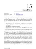
As stated, the PMSM consists of a multiphase stator and a rotor with permanent magnets. The machines

can have either radially or axially oriented flux. Some common radial-flux rotor configurations are depicted
in Fig. 12.1. The magnets can be either mounted on the rotor surface (Fig. 12.1a) or buried in the rotor
iron (Fig. 12.1b). The surface-mounted variety is popular because of the simplicity of construction and
control, and virtual absence of reluctance torque since the stator inductance is essentially independent of
rotor position. The buried magnet (or “interior magnet”) variety of rotors has significant reluctance torque
due to position-variant stator inductance that complicates analysis and control issues. However, the
magnetic saliency can be used advantageously for operation above base speed. There are also variations
of the stator design that are possible, particularly in regard to slot skewing and tooth shape. There is a
wide variety of motor designs, each of which has its own performance and cost considerations.
There are several different magnet materials that are commonly used. Ferrite is an inexpensive but
less magnetically powerful material that is frequently used. The rare earth magnets neodymium-iron-
boron (NdFeB) and samarium-cobalt (SmCo) magnets are stronger magnetically and more resistant to
temperature. SmCo magnets are particularly resistant to temperature but are comparably very expensive.
Sintered NdFeB magnets have a stronger residual field and lower cost than SmCo magnets, but are less
temperature resistant. Bonded NdFeB magnets are not quite as strong as SmCo, but are less expensive
and are more easily shaped. Ferrite magnets are very common for lower-performance motors. Both radial
and parallel magnetization are commonly used, depending on application. The particular choice of
magnets and other design factors is important, but does not directly influence the basic principles of
power converter control.
The multiphase stator is much like the stator of any other AC machine. Frequently, the slot design is
distinctive in that measures are taken to reduce cogging torque. Use of tooth “shoes” and slot skewing is
prevalent. Although distributed windings are common, lumped windings are also used when it is desired
to have an approximately “trapezoidal” back emf. Advances are being made in the area of slotless (i.e.,
“toothless”) PMSM design as well [4].

FIGURE 12.1

Typical PMSM rotor configurations: (a) surface-mount; (b) buried.

© 2002 by CRC Press LLC

The aspects of motor construction that most significantly influence power converter design are the
shape of the back emf, the cogging torque, the magnetic saliency (surface-mount or buried magnets),
and the power requirements. Any of the standard inverter topologies discussed in Chapters 5 and 6
can be used to drive the machine. A conceptual drive system is pictured in Fig. 12.2. There, a speed,
position, or torque command is input to the drive system. The motion controller implements feedback
control based on mechanical sensors (or estimators). The controller outputs commands for the
electrical variables to obey. The electrical control block converts its input commands into commands
for the power converter/modulator block and sometimes utilizes feedback of voltage or current. The
power converter block imposes the desired electrical signals onto the PMSM machine with the
connected load.

12.3 Simulation and Model

When designing a PMSM drive, it is useful to compose a computer simulation before building a prototype.
Such a model can also be used to develop the control. A suitable model of the PMSM is set forth in this
section. Much of the detail of development is omitted because it is not the purpose of this chapter to provide
derivations, but simply to provide the reader with useful formulas for designing the electronics for PMSM
drive systems. Full development of PMSM drive models is available from a number of references [1, 2].
If there are

N

phases, then there are

N

stator voltages, currents, and flux linkages. Let the set of stator
voltages be represented compactly as
(12.1)

where

v

x

is the voltage across the

x

th phase. The same relationship holds for the vectors of current (

i

),
and flux linkage (

λ

). For the special and common case of three-phase machines, the letters

a

,

b

, and

c

are used in place of 1, 2, and 3, respectively, in Eq. (12.1).
Since eddy current and hysteresis losses are generally small, it will suffice to attribute all stator losses
to the winding resistance,

r

. Then, applying Faraday’s and Ohm’s laws, the stator voltage equation may

FIGURE 12.2

Diagram of conceptual drive system.
v v
1
v
2
…
v
N
[]
T
=

© 2002 by CRC Press LLC

be written as
(12.2)
Regarding the machine as balanced, symmetrical, and magnetically linear, the flux linkage equation
may be written as
(12.3)

where

L

is a symmetric

N



×



N

matrix of the appropriate self- and mutual inductances and

λ

pm

is an

N



×

1 vector of stator flux linkages due to the permanent magnet. The inductance matrix is constant for
machines with surface-mounted magnets, but has rotor position–dependent terms for machines with
buried magnets.
The torque equation can be derived from coenergy relationships:
(12.4)
where

θ

r

is the electrical rotor position in radians, and

P

is the number of poles. Mechanical rotor position
is

θ

rm



=

2

θ

r

/

P

. The cogging torque is represented as

T

cog

.
Equations (12.2) to (12.4) represent a simulation model of the machine, provided that the resistance,

r

, the inductance matrix,

L

, the cogging torque,

T

cog

, and the permanent magnet flux linkage vector,

λ

pm

,
are known. The parameters can be determined from direct measurement or by calculation from motor
geometry (i.e., finite-element analysis). The mechanical dynamics of the system, which are not discussed
here since they can widely vary, must be simulated to determine position and speed.
The model set forth is general for any number of phases and for the buried or surface-mounted magnet
cases. For a surface-mounted magnet machine, the air gap is effectively very wide and uniform since the
magnet material has a relative permeability near 1. This results in stator inductance, which is generally
not dependent upon rotor position. In both the surface-mount and buried magnet cases,

λ

pm

is a function
of rotor position. Therefore, the torque equation for the surface-mounted case is
(12.5)
and the torque equation for a machine with buried magnets is
(12.6)
where it is noted that the current,

i

, is not explicitly dependent on rotor position.
The cogging torque may be represented as
(12.7)
where

Z

is the set of natural numbers such that the Fourier series constants and are negligible
and the constant,

N

t

, is the number of stator teeth. The cogging torque is frequently ignored in designing
the motor drive electronics or it is sufficiently negligible because of special machine design efforts. If
cogging torque is neglected, then the constants and are zero.
v ri
d
dt
-----
l+=
l Li l
pm
+=
T
e
P
2
---
∂
∂q
r
-------
1

2
--
i
T
Li i
T
l
pm
+


T
cog
+=
T
e SM()
P
2
---
i
T
∂
∂q
r
-------
l
pm
T
cog
+=

T
e BM()
P
2
---
i
T
1
2
--
∂
∂q
r
-------
L


i
∂
∂q
r
-------
l
pm
+


T
cog
+=

T
cog
T
q
z
zN
t
q
r
()T
d
z
zN
t
q
r
()sin+cos
z∈Z
∑
=
T
q
z
T
d
z
T
q
z
T

d
z

© 2002 by CRC Press LLC

The power into the machine is simply the sum of the power into each phase:
(12.8)
and the power output of the machine is
(12.9)
where

ω

rm

is the mechanical rotor speed. In Eq. (12.9), the frictional and windage dynamics are assumed
to be negligible or to be accounted for in the mechanical system model.
As a common special case of the model in Eq. (12.9), the analysis is restricted to three-phase machines
(

N



=

3). Frequently, the back emf of the machine has negligible harmonics, and thus it can be treated as
if it is purely sinusoidal. As is common in buried magnet machine analysis, the rotor position variance
of the stator inductance can be taken as sinusoidal. Furthermore, the cogging torque can be made small
by utilizing certain design techniques. With these assumptions, a transformation of machine variables

into the rotor reference frame can be made that facilitates vector control of the PMSM.
If the back emf is sinusoidal, then the flux linkage due the permanent magnets is as well. That is,

λ

pm

may be expressed as
(12.10)
where

λ

m

is a constant equal to the peak strength of the flux linkage due to the magnets. Note that
Eq. (12.10) implies a certain interpretation of the measured rotor position. Specifically, it implies that
the magnet flux linking the first phase is zero when

θ

r



=

0. Then, the back emf due to the permanent
magnets may be stated as
(12.11)

where

ω

r

is the electrical rotor speed and equals

P

/2 times its mechanical counterpart,

ω

rm

. Equation (12.11)
is a useful expression for determining the constant

λ

m

experimentally.
The rotor position–dependent terms can be eliminated by transforming the variables into a reference
frame fixed in the rotor. Only the results of this long process are given here. The transformation is applied
as
(12.12)
where
(12.13)

and [Ref. 1]
(12.14)
P
in
v
T
i=
P
out
T
e
w
rm
=
l
pm
l
m
q
r
() q
r
2p
3
------–


q
r
2p

3
------
+


sinsinsin
T
=
e
pm
w
r
l
m
q
r
()cos q
r
2p
3
------–


q
r
2p
3
------
+



coscos
T
=
v
qd0
Kv=
v
qd0
v
q
v
d
v
0
[]
T
=
K
2
3
--
q
r
()cos q
r
2p
3
------–



cos q
r
2p
3
------
+


cos
q
r
()sin q
r
2p
3
------–


sin q
r
2p
3
------
+


sin
1
2

--
1
2
--
1
2
--
=