Streaming Potential in Unconsolidated Samples Saturated with Monovalent Electrolytes
Bạn đang xem bản rút gọn của tài liệu. Xem và tải ngay bản đầy đủ của tài liệu tại đây (2.21 MB, 11 trang )
<span class='text_page_counter'>(1)</span><div class='page_container' data-page=1>
Streaming Potential in Unconsolidated Samples
Saturated with Monovalent Electrolytes
Luong Duy Thanh
1,*<sub>, Rudolf Sprik</sub>
2<i>1<sub>Thuy Loi University, 175 Tay Son, Dong Da, Hanoi, Vietnam</sub></i>
<i>2<sub>Van der Waals-Zeeman Institute, University of Amsterdam, The Netherlands</sub></i>
Received 30 July 2017
Revised 22 September 2018; Accepted 22 September 2018
<b>Abstract: The streaming potential coefficient of liquid-rock systems is theoretically a very</b>
complicated function depending on many parameters including temperature, fluid concentration,
fluid pH, as well as rock parameters such as porosity, grain size, pore size, and formation factor
etc. At a given porous media, the most influencing parameter is the fluid conductivity or
electrolyte concentration. Therefore, it is useful to have an empirical relation between the
streaming potential coefficient and electrolyte concentration. In this work, the measurements of the
streaming potential for four unconsolidated samples (sandpacks) saturated with four monovalent
electrolytes at six different electrolyte concentrations have been performed. From the measured
streaming potential coefficient, the empirical expression between the streaming potential
coefficient and electrolyte concentration is obtained. The obtained expression is in good agreement
with those available in literature. Additionally, it is seen that the streaming potential coefficient
depends on types of cation in electrolytes and on samples. The dependence of the streaming
potential coefficient on types of cation is qualitatively explained by the difference in the binding
constant for cation adsorption on the silica surfaces. The dependence of the streaming potential
coefficient on samples is due to the variation of effective conductivity and the zeta potential
between samples.
<i><b>Keywords: Streaming potential coefficient, zeta potential, porous media, sands. </b></i>
<b>1. Introduction</b>
The streaming potential is induced by the relative motion between the fluid and the solid surface.
In porous media such as rocks, sands or soils, the electric current density, linked to the ions within the
fluid, is coupled to the fluid flow. Streaming potential plays an important role in geophysical
applications. For example, the streaming potential is used to map subsurface flow and detect
subsurface flow patterns in oil reservoirs [e.g., 1]. Streaming potential is also used to monitor
<sub>Corresponding author. Tel.: 84-936946975.</sub>
Email:
</div>
<span class='text_page_counter'>(2)</span><div class='page_container' data-page=2>
subsurface flow in geothermal areas and volcanoes [e.g., 2, 3]. Monitoring of streaming potential
anomalies has been proposed as a means of predicting earthquakes [e.g., 4, 5] and detecting of seepage
through water retention structures such as dams, dikes, reservoir floors, and canals [6].
The streaming potential coefficient (SPC) is a very important parameter, since this parameter
controls the amount of coupling between the fluid flow and the electric current flow in porous media.
The SPC of liquid-rock systems is theoretically a very complicated function depending on 18
fundamental parameters including temperature, pore fluid concentration, fluid pH, as well as rock
parameters such as porosity, grain size, pore size, and formation factor etc [e.g., 7, 8]. At a given
porous media, the most influencing parameter is the fluid conductivity. Therefore, it is useful to have
an empirical relation between the SPC and fluid conductivity or electrolyte concentration. For
example, Jouniaux and Ishido [8] obtain an empirical relation to predict the SPC from fluid
conductivity based on numerous measurements of the streaming potential on sand saturated by NaCl
which have been published. By fitting experimental data collected for sandstone, sand, silica
nanochannels, Stainton, and Fontainebleau with electrolytes of NaCl and KCl, Jaafar et al. [9] obtain
another empirical expression between the SPC and electrolyte concentration. However, experimental
data sets they used for fitting are from different sources with dissimilar fluid conductivity, fluid pH,
temperature, mineral composition of porous media. All those dissimilarities may cause the empirical
expressions less accurate. To critically seek empirical expressions to estimate the SPC from electrolyte
concentration, we have carried out streaming potential measurements for a set of four sandpacks
saturated by four monovalent electrolytes (NaCl, NaI, KCl and KI) at six different electrolyte
concentrations (10−4<sub> M, 5.0×10</sub>−4<sub> M, 10</sub>−3<sub> M, 2.5×10</sub>−3<sub> M, 5.0×10</sub>−3<sub> M, and 10</sub>−2<sub> M).</sub>
From the measured SPC, we obtain the empirical expression between the SPC and electrolyte
concentration. The obtained expression is in good agreement with those reported in [8, 9] in which the
SPC in magnitude is inversely proportional to electrolyte concentration. Additionally, it is seen that
the streaming potential coefficient depends on types of cation in electrolytes and on samples. The
dependence of the streaming potential coefficient on types of cation is qualitatively explained by the
difference in the binding constant for cation adsorption on the silica surfaces. The dependence of the
streaming potential coefficient on samples is due to the variation of effective conductivity and the zeta
potential between samples.
This paper includes five sections. Section 2 describes the theoretical background of streaming
potential. Section 3 presents the experimental measurement. Section 4 contains the experimental
results and discussion. Conclusions are provided in the final section.
<b>2. Theoretical background of streaming potential </b>
<i>2.1. Electrical Double Layer</i>
</div>
<span class='text_page_counter'>(3)</span><div class='page_container' data-page=3>
in one dimension perpendicular to a broad planar interface is well-known and produces an electric
potential profile that decays approximately exponentially with distance as shown in Fig. 1. In the bulk
liquid, the number of cations and anions is equal so that it is electrically neutral. The closest plane to
the solid surface in the diffuse layer at which flow occurs is termed the shear plane or the slipping
plane, and the electrical potential at this plane is called the zeta potential (ζ). The zeta potential plays
an important role in determining the degree of coupling between the electric flow and the fluid flow in
porous media. Most reservoir rocks have a negative surface charge and a negative zeta potential when
in contact with ground water [13, 14]. The characteristic length over which the EDL exponentially
decays is known as the Debye length and is on the order of a few nanometers in most rock-water
systems. The Debye length is a measure of the diffuse layer thickness; its value depends solely on the
properties of the fluid and not on the properties of the solid surface [15] and is given by (for a
symmetric, monovalent electrolyte such as NaCl)
<i>o r b</i>
<i>d</i> <i>2</i>
<i>f</i>
<i>k T</i>
<i>2000Ne C</i>
, (1)
<i>where kb is the Boltzmann’s constant, ε0 is the dielectric permittivity in vacuum, εr</i> is the relative
<i>permittivity of the fluid, T is temperature (in K), e is the elementary charge, N is the Avogadro’s</i>
<i>number and Cf</i> is the electrolyte concentration (mol/L).
Figure 1. Stern model [10, 11] for the charge and electric potential distribution in the electric double layer at a
solid-liquid interface. In this figure, the solid surface is negatively charged and the mobile counter-ions in the
diffuse layer are positively charged (in most rock-water systems).
Figure 2. Development of streaming potential when an electrolyte is pumped through a capillary (a porous
medium is made of an array of parallel capillaries).
</div>
<span class='text_page_counter'>(4)</span><div class='page_container' data-page=4>
The different flows (fluid flow, electrical current flow, heat flow etc.) are coupled by the general
equation
<b>J</b><i>i</i> =
<i>n</i>
<i>ij</i>
<i>j 1</i>
<i>L</i>
<b>X</b><i>j</i>, (2)
<b>which links the forces X</b><i>j </i><b> to the macroscopic fluxes J</b><i>i through transport coupling coefficients Lij</i>
[16].
Considering the coupling between the hydraulic flow and the electric current flow, assuming a
<b>constant temperature and no concentration gradients, the electric current density J</b>e (A/m2) and the flow
<b>of fluid J</b>f (m/s) can be written as the following coupled equation [e.g., 8]:
<b>J</b>e =- <i>0</i> <i>V</i> <i>Lek</i><i>P.</i> (3)
<b>J</b>f =-
<i>0</i>
<i>ek</i>
<i>k</i>
<i>L</i> <i>V</i> <i>P,</i>
(4)
<i>where P is the pressure that drives the fluid flow (Pa) , V is the electrical potential (V), </i> is the<i>0</i>
bulk electrical conductivity, <i>k is the bulk permeability (m0</i> 2), is the dynamic viscosity of the fluid
(Pa.s), and <i>L is the electrokinetic coupling (A.Paek</i> -1.m-1). The first term in Eq. (3) is the Ohm’s law,
<i>and the second term in Eq. (4) is the Darcy’s law. The coupling coefficient L</i>ek is the same in Eq. (3)
and Eq. (4) because the coupling coefficients must satisfy the Onsager’s reciprocal relation in the
steady state. From these equations, it is possible to notice that even if no potential difference is applied
<i>( V = 0), then simply the presence of a pressure difference can produce an electric current. On the</i>
other hand, if no pressure difference is applied (<i>P = 0), the presence of an electric potential</i>
difference can still generate a fluid flow by electroosmosis.
<b>The SPC (V/Pa) is defined when the electric current density J</b>e is zero, leading to
<i>ek</i>
<i>S</i>
<i>0</i>
<i>L</i>
<i>V</i>
<i>C</i> <i>.</i>
<i>P</i>
(5)
<i>This coefficient can be measured by applying a pressure difference ∆P to a porous medium and by</i>
<i>detecting the induced electric potential difference ∆V (see Fig. 2). The driving pressure induces a</i>
streaming current (second term in Eq. (3)) which is balanced by the conduction current (first term in
Eq. (3)) which leads to the electric potential difference that can be measured. In the case of a
unidirectional flow through a cylindrical saturated porous rock, this coefficient can be expressed as
[e.g., 1, 4, 8]
<i>r o</i>
<i>S</i>
<i>eff</i>
<i>C</i> <i>,</i>
(6)
<i>where σeff is the effective conductivity, and ζ is the zeta potential. The effective conductivity</i>
includes the fluid conductivity and the surface conductivity. To characterize the relative contribution
of the surface conductivity, the dimensionless quantity called the Dukhin number has been introduced
[17]. The SPC can also be written as [e.g., 8, 18]
</div>
<span class='text_page_counter'>(5)</span><div class='page_container' data-page=5>
<i>where σr is the electrical conductivity of the sample saturated by a fluid with a conductivity of σf</i>
<i>and F is the formation factor. The electrical conductivity of the sample can possibly include surface</i>
conductivity. If the fluid conductivity is much higher than the surface conductivity, the effective
<i>conductivity is approximately equal to the fluid conductivity, σeff = Fσr = σf</i> and the SPC becomes the
well-known Helmholtz-Smoluchowski equation:
<i>r o</i>
<i>S</i>
<i>f</i>
<i>C</i> <i>.</i>
(8)
<b>3. Experiment</b>
Streaming potential measurements have been performed on four unconsolidated samples of sand
particles with different diameters (See Table 1). The samples are made up of blasting sand particles
obtained from Unicorn ICS BV Company. Four monovalent electrolytes (NaCl, NaI, KCl and KI) are
used with 6 different concentrations (10−4<sub> M, 5.0×10</sub>−4<sub> M, 10</sub>−3<sub> M, 2.5×10</sub>−3<sub> M, 5.0×10</sub>−3<sub> M, and 10</sub>−2
M). All measurements are carried out at room temperature (22 ±1o<sub>C).</sub>
<i>3.1. Sample Assembly</i>
Samples are constructed by filling polycarbonate plastic tubes (1 cm in inner diameter and 7.5 cm
in length) successively with 2 cm thick layers of particles that are gently tamped down, and they are
then shaken by a shaker (TIRA-model TV52110). Filter paper is used in both ends of the tube to retain
the particles and is permeable enough to let the fluid pass through. The samples are flushed with
distilled water to remove any powder or dust.
<i>3.2. Porosity, Permeability, and Formation Factor Measurements</i>
The porosity is measured by a simple method mentioned in [19] and reference therein. The sample
is first dried in oven for 24 hours, then cooled to room temperature, and finally fully saturated with
<i>deionized water under vacuum. The sample is weighed before (mdry) and after full saturation (mwet</i>) by a
vacuum desiccator and the porosity is determined as
<i>wet</i> <i>dry</i>
<i>( m</i> <i>m ) /</i>
<i>,</i>
<i>AL</i>
(9)
<i>where ρ is density of the water, A and L are the cross sectional area and the physical length of the</i>
samples, respectively. The measured porosity of the samples is 0.39 independently of the size of sand
particles with an error of 5%. This value is in good agreement with [20] for a random packing of
spherical particles.
<i>Table 1. Sample ID, diameter range, permeability ko, porosity, formation factor F and tortuosity α∞</i>.
Sample ID Size (μm) <i>ko</i>(m2) <i>F</i> <i>α∞</i>
1 S1 300-400 13.2×10⁻¹² <sub>4.2</sub> <sub>1.64</sub>
2 S2 200-300 7.5×10⁻¹² <sub>4.0</sub> <sub>1.56</sub>
3 S3 90-150 3.8×10⁻¹² <sub>4.2</sub> <sub>1.64</sub>
</div>
<span class='text_page_counter'>(6)</span><div class='page_container' data-page=6>
<b>Figure 3. The flow rate against pressure difference. Two runs are shown for the sample S3.</b>
Permeability is determined by a constant flow-rate experiment (see [19] and reference therein for
more details). A high pressure pump (LabHut, Series III- Pump) ensures a constant flow through the
sample, a high precision differential pressure transducer (Endress and Hauser Deltabar S PMD75) is
used to measure the pressure drop. For low velocities Darcy’s law holds
<i>o</i>
<i>f</i>
<i>k A P</i>
<i>Q</i> <i>,</i>
<i>L</i>
(10)
<i>where Qf is the fluid volume flow rate, ko is the permeability, ∆P is the differential pressure</i>
<i>imposed across the sample, η is the viscosity of the fluid. The permeability is then determined from</i>
the slope of the flow rate - pressure graph (see Figure 3 for the sample S3, for example) with the
<i>knowledge of L, A and η (10</i>-3<sub> Pa.s). The graph shows that there is a linear relationship between flow</sub>
rate and pressure difference and Darcy’s law is obeyed. Similarly, the permeability of other samples is
obtained and reported in Table 1 with an error of 10 %.
Figure 4. Schematic of the experimental setup to measure the saturated sample resistance.
Method of determining the formation factor and tortuosity is introduced in [19] and reference
<i>therein. The formation factor F is defined as:</i>
<i>f</i>
<i>r</i>
<i>F</i> <i>,</i>
</div>
<span class='text_page_counter'>(7)</span><div class='page_container' data-page=7>
<i>where α∞ is the tortuosity, ϕ is the porosity of the sample, σf</i> is the electrical conductivity of the
<i>fluid directly measured by a conductivity meter (Consort C861) and σr</i> is the electrical conductivity of
the fully saturated sample. Eq. (11) is only valid when surface conductivity effects become negligible
<i>(σf </i>is higher than 0.60 S/m as stated in [21] for silica-based samples). Schematic of the experimental
setup to measure resistances of saturated samples is shown in Figure 4. The electrodes for the
resistance measurements are silver meshes. The electrodes are placed on both sides against the sample
that is fully saturated successively with a set of NaCl solutions with high conductivities. The sample
<i>resistance is measured by an impedance analyzer (Hioki IM3570) to calculate σr</i> with the knowledge
<i>of the geometry of the sample (the length and the diameter). From the measured values of σf and σr</i>,the
formation factor and corresponding tortuosity are determined with an error of 6 % and 9 %,
respectively (see Table 1). The measured formation factors of the samples are the range from 4.0 to
4.3. According to Archie’s law, <i>F</i><i>m in which is the porosity of the sample and m is the so</i>
called cementation exponent. For unconsolidated samples made of spherical particles, the exponent is
around 1.5 [22]. Therefore, the measured formation factors are in good agreement with Archie’s law.
Figure 5. Experimental setup for streaming potential measurements.
Figure 6. Streaming potential as a function of pressure difference for the sample S3 and electrolyte KCl at a
concentration of 2.5×10⁻³<sub> M. Three representative measurements are shown.</sub>
</div>
<span class='text_page_counter'>(8)</span><div class='page_container' data-page=8>
The experimental setup for the streaming potential measurement is shown in Fig. 5. The solution
is circulated through the samples until the electrical conductivity and pH of the solution reach a stable
value measured by a multimeter (Consort C861). The pH values of equilibrium solutions are in the
range 6.0 to 7.5. Electrical potential differences across the samples are measured by a high input
impedance multimeter (Keithley Model 2700) connected to a computer and controlled by a Labview
program (National Instruments). Pressure differences across a sample are measured by a
high-precision differential pressure transducer (Endress and Hauser Deltabar S PMD75).
<b>Table 2. The streaming potential coefficient (in mV/bar) for different electrolyte concentrations.</b>
Sample ID Electrolyte 10−4<sub> M</sub> <sub>5.0×10</sub>−4<sub> M</sub> <sub>10</sub>−3<sub> M</sub> <sub>2.5×10</sub>−3<sub> M</sub> <sub>5.0×10</sub>−3<sub> M</sub> <sub>10</sub>−2<sub> M</sub>
S1
NaCl -1250 -202 -120 -41 -20
NaI -1275 -206 -125 -44 -22
KCl -1033 -183 -91 -30 -11
KI -1233 -200 -118 -38 -19
S2
NaCl -1950 -380 -179 -70 -32
NaI -2067 -403 -185 -87 -35
KCl -1230 -263 -127 -58 -26
KI -1700 -350 -170 -60 -27
S3
NaCl -2100 -625 -357 -145 -63 -31
NaI -2466 -763 -400 -160 -77 -34
KCl -1567 -570 -313 -120 -65 -25
KI -1665 -573 -330 -123 -58 -26
S4
NaCl -4021 -842 -429 -149 -69 -33
NaI -4067 -850 -435 -151 -81 -36
KCl -2333 -576 -290 -106 -71 -29
KI -3933 -836 -430 -147 -75 -31
The way used to collect the SPC is already described in [23] and reference therein. Streaming
potential across the sample (ΔV) is measured as a function of applied pressure difference (ΔP). The
SPC is then obtained as the slope of the straight line (see Fig. 6). Three measurements are performed
to find the average value of the SPC. The SPC for all samples at different electrolyte concentrations is
shown in Table 2 except for two samples S1 and S2 at electrolyte concentration of 10-2<sub> M. Because</sub>
these samples are very permeable, they need a very large flow rate to generate measurable electric
potentials at high electrolyte concentration. The maximum error of the SPC is 10 %. It is found that
the SPC is negative for all samples and all electrolytes used in this work.
<b>4. Results and discussion</b>
</div>
<span class='text_page_counter'>(9)</span><div class='page_container' data-page=9>
The experimental results also show that anions have only a small effect on the SPC as observed in
[24].
Figure 7. The magnitude of the SPC as a function of electrolyte concentration
for different electrolytes and for the sample S3.
Fig. 8 shows the variation of the SPC with samples for electrolyte NaI, for example. It is seen that
at a given electrolyte concentration, the SPC depends on the samples. Namely, the magnitude of the
SPC increases in the order from S1, S2, S3 and S4 respectively. This may be due to the variation of
effective conductivity with particle size of the samples and the difference in the zeta potential between
the samples.
From Table 2, the magnitude of the SPC as a function of electrolyte concentration is plotted for all
samples saturated by different electrolytes (see Fig. 9). By fitting the experimental data shown by the
solid line in Fig. 9, the empirical relation between the SPC in magnitude and electrolyte concentration
is obtained as
<i>9</i>
<i>S</i>
<i>f</i>
<i>2.0 10</i>
<i>C</i>
<i>C</i>
(V/Pa) (12)
<i>where Cf</i> is electrolyte concentration.
Figure 8. The magnitude of the SPC as a function of electrolyte concentration for different samples saturated by
electrolyte NaI.
Expression in Eq. (12) has the similar form as the empirical expression
<i>9</i> <i>0.9123</i>
<i>S</i> <i>f</i>
<i>C</i> <sub></sub><i>1.36 10 / C</i><sub></sub>
</div>
<span class='text_page_counter'>(10)</span><div class='page_container' data-page=10>
Additionally, by fitting experimental data on sand saturated by NaCl at pH = 7-8 which are available
in literature, Jouniaux and Ishido [8] obtain the expression
<i>8</i>
<i>S</i> <i>f</i>
<i>C</i> <sub></sub><i>1.2 10 /</i><sub></sub>
(<i>f</i><sub> is the fluid</sub>
conductivity). The relation between fluid conductivity of a NaCl solution and electrolyte concentration
in the range 10-6<i><sub>M < C</sub></i>
<i>f</i> < 1 M (15oC < temperature < 25oC) is given as <i>f</i> <i>10Cf</i>[25]. Therefore, we
get the expression
<i>9</i>
<i>S</i> <i>f</i>
<i>C</i> <sub></sub><i>1.2 10 / C</i><sub></sub>
based on [8] and that is also similar to Eq. (12). The prediction
of SPC as a function of electrolyte concentration from the empirical expressions of [8, 9] is also shown
in Fig. 9 (see the dashed lines). It is seen that the predictions from [8, 9] have the same behavior as
that obtained in this work but give smaller values of the SPC at a given electrolyte concentration. The
reason for the deviation between the empirical expressions may be due to dissimilarities of fluid
conductivity, fluid pH, mineral composition of porous media, temperature etc.
Figure 9. SPC in magnitude as a function of electrolyte concentration for different samples (S1, S2, S3 and S4)
and different electrolytes (NaCl, NaI, KCl and KI). Symbols are experimental data. Solid line is the fitting line
and two other dashed lines are predicted from [8] and [9].
<b>5. Conclusions</b>
</div>
<span class='text_page_counter'>(11)</span><div class='page_container' data-page=11>
<b>Acknowledgments</b>
The first author would like to thank Vietnam National Foundation for Science and Technology
Development (NAFOSTED) under grant number 103.99-2016.29 for the financial support.
<b>References</b>
[1] B. Wurmstich, F. D. Morgan, Geophysics 59 (1994) 46–56.
[2] R. F. Corwin, D. B. Hoovert, Geophysics 44 (1979) 226–245.
[3] F. D. Morgan, E. R. Williams, T. R. Madden, Journal of Geophysical Research 94 (1989) 12.449–12.461.
[4] H. Mizutani, T. Ishido, T. Yokokura, S. Ohnishi, Geophys. Res. Lett. 3 (1976).
[5] M. Trique, P. Richon, F. Perrier, J. P. Avouac, J. C. Sabroux, Nature (1999) 137–141.
[6] A. A. Ogilvy, M. A. Ayed, V. A. Bogoslovsky, Geophysical Prospecting 17 (1969) 36–62.
[7] P. W. J. Glover, E. Walker, and M. D. Jackson, Geophysics 77 (2012) D17–D43.
[8] L. Jouniaux and T. Ishido, International Journal of Geophysics, vol. 2012, Article ID 286107, 16 pages, 2012.
doi:10.1155/2012/286107.
[9] Vinogradov, J., M. Z. Jaafar, and M. D. Jackson, Journal of Geophysical Research Atmospheres 115 (2010)
B12204.
[10] O. Stern, Z. Elektrochem 30 (1924) 508–516.
[11] T. Ishido, H. Mizutani, Journal of Geophysical Research 86 (1981) 1763– 1775.
[12] H. M. Jacob, B. Subirm, Electrokinetic and Colloid Transport Phenomena, Wiley-Interscience, 2006.
[13] K. E. Butler, Seismoelectric effects of electrokinetic origin, PhD thesis, University of British Columbia, 1996.
[14] H. Hase, T. Ishido, S. Takakura, T. Hashimoto, K. Sato, Y. Tanaka, Geophysical Research Letters 30 (2003)
3197–3200.
[15] R. J. Hunter, Zeta Potential in Colloid Science, Academic, New York, 1981.
[16] L. Onsager, Physical Review 37 (1931) 405-426.
[17] S. Dukhin, V. Shilov, Dielectric Phenomena and the Double Layer in Disperse Systems and Polyelectrolytes,
John Wiley and Sons, New York, 1974.
[18] L. Jouniaux, M. L. Bernard, M. Zamora, J. P. Pozzi, Journal of Geophysical Research B 105 (2000) 8391–8401.
<i>[19] Luong Duy Thanh, Rudolf Sprik, VNU Journal of Science: Mathematics-Physics 32 (2016) 22-33.</i>
[20] Paul W. Glover and Nicholas Déry. Geophysics 75(2010), F225-F241.
[21] S. F. Alkafeef and A. F. Alajmi, Colloids and Surfaces A 289 (2006) 141–148.
[22] P. N. Sen, C. Scala, and M. H. Cohen, Geophysics 46 (1981) 781–795.
<i>[23] Lưong Duy Thanh, Rudolf Sprik, VNU Journal of Science: Mathematics and Physics 31 (2015) 56-65.</i>
[24] Luong Duy Thanh and Rudolf Sprik (2016). “Zeta potential in porous rocks in contact with monovalent and
divalent electrolyte aqueous solutions” geophysics, 81(4), D303-D314.
</div>
<!--links-->