High-pressure Melting Curves of α and ¥ Phases of Iron
Bạn đang xem bản rút gọn của tài liệu. Xem và tải ngay bản đầy đủ của tài liệu tại đây (832.71 KB, 7 trang )
<span class='text_page_counter'>(1)</span><div class='page_container' data-page=1>
99
Original Article
High-pressure Melting Curves of
and
<sub> Phases of Iron </sub>
Nguyen Thi Hong
1,2,*<sub>, Ho Khac Hieu</sub>
3<i>1<sub>Hong Duc University, Thanh Hoa, Vietnam </sub></i>
<i>2<sub>VNU University of Science, Hanoi, Vietnam </sub></i>
<i>3<sub>Duy Tan University, Da Nang, Vietnam </sub></i>
Received 22 September 2019
<i>Revised 11 October 2019; Accepted 15 October 2019 </i>
<b>Abstract: Statistical moment method (SMM) has been applied in combination with Lindemann </b>
melting criterion to investigate pressure effects on melting temperature of iron. Melting curves of
phase with body-centered cubic structure and
phase with face-centered cubic structure of ironhave been derived up to pressure 13 GPa and 90 GPa, respectively. This work shows that melting
curves of these two phases of iron are increasing functions of pressure, and the higher the pressure
is the lower the slopes of melting curves are. Our results are compared with those of available
experimental data to verify the developed theory. The efficiency of the SMM on the investigation
of melting temperatures of
and
phases of iron allows us to believe that the present SMMscheme can be developed extensively to determine melting temperatures of other phases of iron as
well as other materials.
<i>Keywords: Melting, high pressure, iron, Lindemann criterion, Statistical moment method. </i>
<b>1. Introduction </b>
<i>Earth’s solid inner core is mainly composed of iron [1]. Iron has four main polymorphs including </i>
phase with body-centered cubic (BCC) structure, phase with face-centered cubic (FCC) structure,
phase with hexagonal close-packed (HCP) structure, and
phase with BCC structure at hightemperature [2-4]. Moreover, Andrault et al. experimentally showed the persistence of the fifth phase -
phase of iron at high temperature and pressure [5]. Melting curves of iron in different structural________
<sub>Corresponding author. </sub>
</div>
<span class='text_page_counter'>(2)</span><div class='page_container' data-page=2>
phases at high pressure provide essential information to investigate complex seismic structures inside
the Earth's core [6-7]. The investigation of melting of iron under high pressure has been performed by
<i>different theoretical methods (ab initio calculations [8], molecular dynamic simulations [9], empirical </i>
approach [10-12]) and experimental measurements (laser-heated diamond-anvil cell [13-15], shock
compression [16]). However, up to now, the results obtained from different methods are still not unified.
In this work, by developing the statistical moment method (SMM) in statistical mechanics, we
<i>investigate the pressure dependence of melting temperatures of α and γ phases of iron. The slopes of </i>
melting curves have also been derived. Our numerical calculations are compared with those of previous
theoretical and empirical works to verify the research approach.
<b>2. Theoretical approach </b>
The melting temperature of iron, in present work, is derived based on the Lindemann melting
criterion which was proposed that [17-19]: “Melting of a material is going to occur when the so-called
Lindemann ratio
2
,
,
<i>u</i>
<i>P T</i>
<i>a P T</i>
reaches a threshold value”, where <i>u</i>2 is the atomic mean-square
displacement (MSD) and <i>a P T</i>
,
is the nearest-neighbor distance (NND) between two intermediateatoms.
In order to derive the melting point of iron at different pressures, we propose an assumption that the
Lindemann ratio remains constant for all range of studied pressure [20], i.e.:
<sub></sub>
<sub></sub>
0
2 <sub>,</sub> 2 <sub>0,</sub>
, 0,
, 0,
<i>u</i> <i>P T</i> <i>u</i> <i>T</i>
<i>P T</i> <i>T</i>
<i>a P T</i> <i>a</i> <i>T</i>
,
(1)
where
2
0
0,
0,
0,
<i>u</i> <i>T</i>
<i>T</i>
<i>a</i> <i>T</i>
is the Lindemann ratio at ambient pressure and at melting point
temperature of the material. This assumption can be seen as an expansion of Lindemann criterion. This
comes from a truth that when pressure increases, both MSD and NND quantities will be reduced due to
the limitation of atomic vibrations. Below we present a method to determine the NND <i>a P T</i>
,
andMSD <i>u</i>2 of atoms.
<i>2.1. Nearest-neighbor distance </i>
In SMM approach, the NND <i>a P T was derived as [21] </i>
,
<i>a P,T</i>
<i>a</i><sub>0</sub>
<i>P,</i>0 <i>y</i><sub>0</sub>
<i>P,T</i> , (2)where <i>a</i><sub>0</sub>
<i>P,</i>0 is NND at 0 K,
0
2
2
3
3
<i>y</i> <i>P,T</i> <i>A</i>
<i>k</i>
</div>
<span class='text_page_counter'>(3)</span><div class='page_container' data-page=3>
<i>The parameters A, k, and γ were defined as follows [21] </i>
2 2 3 3 4 4 5 5 6 6
1 4 2 6 3 8 4 10 5 12 6
<i>A a</i>
<i>a</i>
<i>a</i>
<i>a</i>
<i>a</i>
<i>a ,</i>
<i>k</i>
<i>k</i>
<i>k</i>
<i>k</i>
<i>k</i>
2
2
0
0
2
1
2
<i>i</i>
<i>i</i> <i><sub>eq</sub></i>
<i>k</i> <i>m</i> <i>,</i>
<i>i</i> <i>u</i><sub></sub>
(3)4
4
0
4 2 2
1
6
12
<i>i</i>
<i>ix</i> <i>ix</i> <i>iy</i> <i><sub>eq</sub></i>
<i>io</i> <i><sub>,</sub></i>
<i>i</i> <i>u</i> <i><sub>eq</sub></i> <i>i</i> <i>u</i> <i>u</i>
<sub></sub>
<sub></sub>
<sub></sub>
<sub></sub>
<sub></sub>
<sub></sub>
<sub></sub>
<sub></sub>
<sub></sub>
<sub></sub>
<sub></sub>
<sub></sub>
(4)
where
<i>a ,a ,a ,a ,a ,a</i>
<sub>1</sub> <sub>2</sub> <sub>3</sub> <sub>4</sub> <sub>5</sub> <sub>6</sub> were defined as in Ref. [21],
<i><sub>io</sub></i>is the interaction potential between the<i>i</i>th<i><sub> and the 0</sub></i>th<sub> particles, </sub>
0
<i>m</i>
is the atomic mass.The NND
<i>a</i>
<sub>0</sub>
<i>P,</i>
0
can be calculated from the SMM equation-of-state (EOS) as [21]1 0 1
6 2
<i>U</i> <i><sub>k</sub></i>
<i>Pv</i> <i>a</i> <i>X</i>
<i>a</i> <i>k a</i>
<sub></sub>
, (5)
where
<i>v</i>
is the atomic volume,<i>U</i>
<sub>0</sub> is the total potential energy of system, andcoth
2 2
<i>X</i>
<sub></sub> <sub></sub> <sub></sub> <sub></sub>
.
At ambient temperature, the Eq. (5) is reduced to a simple form
1 0 0 <sub>.</sub>
6 4
<i>U</i> <i>k</i>
<i>Pv</i> <i>a</i>
<i>a</i> <i>k</i> <i>a</i>
(6)
In order to perform numerical calculations, we assume the interaction potential between
two intermediate atoms could be described by the Lennard–Jones potential as
0 0 ,<i>n</i> <i>m</i>
<i>r</i> <i>r</i>
<i>D</i>
<i>r</i> <i>m</i> <i>n</i>
<i>n</i> <i>m</i> <i>a</i> <i>a</i>
<sub> </sub>
<sub> </sub>
<sub> </sub>
<sub> </sub>
(7)where
<i>D</i>
describes the dissociation energy,<i>r</i>
<sub>0</sub><i> is the equilibrium value of a, and </i><i>n m</i>
,
aredetermined by fitting experimental data.
Using the coordination sphere method, we derive the total potential energy of system as [22]
<sub>0</sub> . 0 0
2( )
<i>n</i> <i>m</i>
<i>n</i> <i>m</i>
<i>r</i> <i>r</i>
<i>N D</i>
<i>U</i> <i>mA</i> <i>nA</i>
<i>n</i> <i>m</i> <i>a</i> <i>a</i>
<sub> </sub>
<sub> </sub>
<sub> </sub>
<sub> </sub>
, (8)where
<i>N</i>
is the total number of particles in the crystal.Substituting
<i>r</i>
of the Lennard-Jones potential into Eqs. (3) and (4), the parameters<i>k</i>
and</div>
<span class='text_page_counter'>(4)</span><div class='page_container' data-page=4>
2
ix
2
ix
0
4 2
2
0
4 2
2
2
2 ,
<i>n</i>
<i>n</i> <i>n</i>
<i>m</i>
<i>m</i> <i>m</i>
<i>r</i>
<i>Dnm</i> <i><sub>a</sub></i>
<i>k</i> <i>n</i> <i>A</i> <i>A</i>
<i>a</i> <i>n</i> <i>m</i> <i>a</i>
<i>r</i>
<i>a</i>
<i>m</i> <i>A</i> <i>A</i>
<i>a</i>
<sub> </sub>
<sub> </sub>
<sub> </sub>
<sub></sub>
<sub> </sub>
(9)
2 2
4 2
ix
ix ix
2 2
4
ix
ix
2
ix
8 8 6
4
0
4 8 8
0
6 4
( 2)( 4)( 6) 6 18( 2)( 4)
12 ( )
9( 2) ( 2)( 4)( 6) 6
18( 2)( 4) 9( 2) ,
<i>iy</i>
<i>iy</i>
<i>n</i> <i>n</i> <i>n</i>
<i>n</i>
<i>n</i> <i>m</i> <i>m</i>
<i>m</i>
<i>m</i> <i>m</i>
<i>Dmn</i> <i><sub>n</sub></i> <i><sub>n</sub></i> <i><sub>n</sub></i> <i><sub>A</sub>a</i> <i><sub>A</sub>a a</i> <i><sub>n</sub></i> <i><sub>n</sub></i> <i><sub>A</sub>a</i>
<i>a n</i> <i>m</i>
<i>r</i> <i>a</i> <i>a a</i>
<i>n</i> <i>A</i> <i>m</i> <i>m</i> <i>m</i> <i>A</i> <i>A</i>
<i>a</i>
<i>r</i>
<i>a</i>
<i>m</i> <i>m</i> <i>A</i> <i>m</i> <i>A</i>
<i>a</i>
<sub></sub> <sub></sub> <sub></sub>
<sub></sub>
<sub></sub>
<sub> </sub> <sub></sub>
(10)
where
2 2
<i>ix</i> <i>ix</i>
<i>a</i> <i>a</i>
<i>n</i> <i>m</i> <i>m</i> <i>n</i>
<i>A , A , A , A</i>
,... are the structural sums of the given crystal [21,22].The EOS of crystal at zero temperature is obtained as [21]
2 2
ix ix
2 2
ix ix
0 0
2
0 0
4 2 4 2
0 0
4 2 4 2
6( ) 4 2
2 2 2 2
.
2 2
<i>n</i> <i>m</i>
<i>n</i> <i>m</i>
<i>n</i> <i>m</i>
<i>n</i> <i>n</i> <i>m</i> <i>m</i>
<i>n</i> <i>m</i>
<i>n</i> <i>n</i> <i>m</i> <i>m</i>
<i>r</i> <i>r</i>
<i>Dnm</i> <i>Dnm</i>
<i>Pv</i> <i>A</i> <i>A</i>
<i>n</i> <i>m</i> <i>a</i> <i>a</i> <i>a</i> <i>M</i> <i>n</i> <i>m</i>
<i>r</i> <i>r</i>
<i>a</i> <i>a</i>
<i>n</i> <i>n</i> <i>A</i> <i>A</i> <i>m</i> <i>m</i> <i>A</i> <i>A</i>
<i>a</i> <i>a</i>
<i>r</i> <i>r</i>
<i>a</i> <i>a</i>
<i>n</i> <i>A</i> <i>A</i> <i>m</i> <i>A</i> <i>A</i>
<i>a</i> <i>a</i>
<sub> </sub> <sub> </sub>
<sub> </sub> <sub> </sub>
<sub> </sub> <sub> </sub>
<sub> </sub> <sub> </sub>
<sub> </sub> <sub> </sub>
<sub> </sub> <sub> </sub>
(11)
This equation can be re-written in a simpler form
4 4
3 3 3 4
1 2
5 6
0 ,
<i>n</i> <i>m</i>
<i>n</i> <i>m</i>
<i>n</i> <i>m</i>
<i>c y</i> <i>c y</i>
<i>c y</i> <i>c y</i> <i>Pv</i>
<i>c y</i> <i>c y</i>
<sub></sub> <sub></sub> <sub></sub> <sub></sub>
(12)
where
2
ix
2
ix
2 2
ix ix
0
1 2
3 4 2
4 4 2
5 4 2 6 4 2
; ; ;
6 6
1
2 2 ;
2
4
1
2 2 ;
2
4
2 ; 2 ;
<i>n</i> <i>m</i>
<i>n</i> <i>n</i>
<i>m</i> <i>m</i>
<i>n</i> <i>n</i> <i>m</i> <i>m</i>
<i>r</i> <i>Dnm</i> <i>Dnm</i>
<i>y</i> <i>c</i> <i>A</i> <i>c</i> <i>A</i>
<i>a</i> <i>n</i> <i>m</i> <i>n</i> <i>m</i>
<i>Dnm</i> <i><sub>a</sub></i>
<i>c</i> <i>n</i> <i>n</i> <i>A</i> <i>A</i>
<i>a</i> <i>M</i> <i>n</i> <i>m</i>
<i>Dnm</i> <i><sub>a</sub></i>
<i>c</i> <i>m</i> <i>n</i> <i>A</i> <i>A</i>
<i>a</i> <i>M</i> <i>n</i> <i>m</i>
<i>a</i> <i>a</i>
<i>c</i> <i>n</i> <i>A</i> <i>A</i> <i>c</i> <i>m</i> <i>A</i> <i>A</i>
3
0
4
3 3
<i>r</i>
(for BCC structure) and 3
0
2
2 <i>r</i>
</div>
<span class='text_page_counter'>(5)</span><div class='page_container' data-page=5>
By numerically solving Eq. (12), we can determine the value of NND <i>a</i><sub>0</sub>
<i>P,</i>0 .<i>2.2. Atomic mean-square displacement </i>
The MSD function can be derived from the second order moment of SMM method as [23]
<i>u</i>2 <i>u</i> 2 <i>A</i><sub>1</sub>
<i>X</i> 1
<i>k</i>
, (13)
where
0
2 2
1 4
,
1 2
1 1 1 .
2
<i>u</i> <i>y</i>
<i>X</i>
<i>A</i> <i>X</i>
<i>k</i> <i>k</i>
<sub></sub>
<sub></sub>
<sub></sub>
<sub></sub>
(14)
<b>3. Results and discussion </b>
In this section, numerical calculations will be performed to evaluate the pressure-dependent melting
<i>temperatures of α and γ phases of iron. The Lennard-Jones potential parameters of iron metal are m = </i>
<i>3.54, n = 6.45, r0 = 2.48 Å, D = 12576.7 kB</i> [23]. With the assumption that the interatomic potential
does not depend on the structure of iron, the above potential could be used for numerical calculations of
<b>these two phases of iron. </b>
<i>In order to determine the melting curves of α (in the pressure range 0–13 GPa) and γ (in the pressure </i>
range 13–90 GPa) phases of iron, we calculate firstly the Lindemann ratio at zero pressure and at melting
point (<i>T<sub>m</sub></i><sub>0</sub> 1811 K). The Lindemann ratios of two phases are obtained, respectively, as <i>0.0589046</i>
and <i>0.0525603 for α-Fe and </i>
-Fe. From these results and from our assumption (the pressureindependence of Lindemann criterion) we derive the melting temperatures of iron at different pressures.
<i>Our melting curves of α and γ phases of iron are shown in Fig. 1. </i>
Fig. 1. Melting curves of α and γ phases of iron. Our results (solid lines) are compared with those of
measurements performed by Anderson [3], Ahrens et al. [24], Komabayashi et al. [25], Jackson et al. [26], and
Sinmyo et al. [27].
</div>
<span class='text_page_counter'>(6)</span><div class='page_container' data-page=6>
<i>As observed from Fig. 1, the melting curves of α and γ phases of iron are increasing functions of </i>
pressure. Our calculations of melting temperatures of iron are reasonably consistent with most of those
of previous works but they overestimate the measurements performed by Komabayashi et al. [25]. The
maximum difference between our predictions and previous works is about 11.68% at 52 GPa.
Especially, it should be noted that our theoretical melting curves are in good agreement with the most
recently published data measured by Sinmyo et al. [27].
<i>We make a futher step by considering the slopes of melting curves of α and γ phases of iron. The </i>
slopes of these two melting curves are presented in Fig. 2. As it can be seen from this figure that the
higher the pressure is the lower the slopes of melting are. Interestingly, at the pressure of structural phase
transition, we can observe the apparent break between two melting curves. The difference between the
slopes of two melting curves at pressure 13 GPa is about 2.2 K/GPa. This break behavior can be applied
for the investigation of the structural phase transition of materials under pressure.
<i>Fig. 2. The slopes of the melting curves of α and γ phases of iron. </i>
<b>4. Conclusions </b>
In this work, we have studied the melting curves of <i>α and γ phases of iron by using the combination </i>
of SMM with modified Lindemann criterion of melting. The slopes of melting curves of these two
phases of iron have also been derived. Our numerical calculations show that the SMM melting
temperatures of these two phases of iron are in reasonable agreement with the available experimental
data. This confirms that our approach has a potential to study pressure effects on melting curves of other
phases of iron as well as other materials.
<b>Acknowledgments </b>
</div>
<span class='text_page_counter'>(7)</span><div class='page_container' data-page=7>
<b>References </b>
[1] Y. Mori, H. Ozawa, K. Hirose, R. Sinmyo, S. Tateno, G. Morard, Y. Ohishi, Melting experiments on Fe–Fe3S
system to 254 Gpa, <b>Earth Planet. Sci. Lett. 464 (2017) 135–141. </b>
[2] C. S. Yoo, J. Akella, A. J. Campbell, H. K. Mao, R. J. Hemley, Phase Diagram of lron by in Situ X-ray Diffraction:
Implications for Earth's Core,Science 270 (1995) 1473-1475.
[3] O. L. Anderson, Iron: Beta Phase Frays, Science 278 (1997) 821-822.
[4] K. Ohta, Y. Kuwayama, K. Shimizu, T. Yagi, K. Hirose, Y. Ohishi, Measurements of electrical and thermal
conductivity of iron under Earth’s core conditions, AGU abstract MR21B-06, AGU Fall Meeting, San Francisco,
(2014) Dec 15–19.
[5] D. Andrault, G. Fiquet, M. Kunz, F. Visocekas, D. Hausermann, The Orthorhombic Structure of iron: An in Situ
<i>Study at High-Temperature and High-pressure , Science 278 (1997) 831. </i>
[6] M. Mattesini, A. B. Belonoshko, E. Buforn, M. Ramírez, S. I. Simak, A. Udías, H. K. Mao, and R. Ahuja,
<i>Hemispherical anisotropic patterns of the Earth’s inner core, Proc. Natl. Acad. Sci. U.S.A. 107 (2010) 9507-9512. </i>
[7] M. Monnereau, M. Calvet, L. Margerin, A. Souriau, Lopsided Growth of Earth's Inner Core, Science 328 (2010)
1014.
[8] A. B. Belonoshko, R. Ahuja, B. Johansson, Stability of the body-centred-cubic phase of iron in the Earth’s inner
core, Nature 424 (2003) 1032.
[9] Y. Wu, L. Wang, Y. Huang, D. Wang, Melting of copper under high pressures by molecular dynamics simulation,
Chem. Phys. Lett. 515 (2011) 217-220.
[10] D. Zhang, J.M. Jackson, J. Zhao, W. Sturhahn, E.E. Alp, M.Y. Hu, T.S. Toellner, C.A. Murphy, V.B. Prakapenka,
Temperature of Earth’s core constrained from melting of Fe and Fe0.9Ni0.1 at high pressures, Earth Planet. Sci. Lett.
447 (2016) 72–83.
[11] H.K. Hieu, Melting of solids under high pressure, Vacuum 109 (2014) 184–186.
[12] H.K. Hieu, T.T. Hai, N.T. Hong, N.D. Sang, N.V. Tuyen, Pressure dependence of melting temperature and shear
modulus of hcp-iron, High Pressure Res. 37 (2017) 267-277.
[13] S. Anzellini, A. Dewaele, M. Mezouar, P. Loubeyre, G. Morard, Diffraction Melting of Iron at Earth's Inner Core
Boundary Based on Fast X-ray, Science 340 (2013) 464–466.
[14] Q. Williams, R. Jeanloz, J. Bass, B. Svendsen, T.J. Ahrens, The Melting Curve of Iron to 250 Gigapascals: A
Constraint on the Temperature at Earth's Center, Science 236 (1987) 181–182.
[15] C.S. Yoo, N.C. Holmes, M. Ross, D.J. Webb, C. Pike, Shock Temperatures and Melting of Iron at Earth Core
Conditions, Phys. Rev. Lett. 70 (1993) 3931–3934.
[16] N.H. Jeffrey, H.C. Neil, Melting of iron at the physical conditions of the Earth’s core, Nature 427 (2004) 339–342.
[17] H.K. Hieu, Volume and pressure-dependent thermodynamic properties of sodium, Vacuum. 120 (2015) 13–16.
[18] H.K. Hieu and N. N. Ha, High pressure melting curves of silver, gold and copper, AIP Adv. 3 (2013) 112125.
[19] F. Lindemann, The calculation of molecular vibration frequencies, Phys. Z. 11 (1910) 609-612.
[20] H.K. Hieu, Systematic prediction of high-pressure melting curves of transition metals, J. Appl. Phys. 116 (2014)
163505-1 - 16305-6.
[21] V.V. Hung, Statistical moment method in studying thermodynamic and elastic property of crystal, HNUE
Publishing House, Hanoi, 2009.
<b>[22] V.V. Hung, N.T. Hoa, Equation of state and thermodynamic properties of BCC metals, ASEAN J. Sci. Tech. Dev. </b>
23 (2006) 27-42.
[23] M. Magomedov, The Calculation of the Parameters of the Mie–Lennard-Jones Potential, High Temp. 44 (2006)
513-529.
[24] T.J. Ahrens, K.G. Holland, G.Q. Chen, Phase diagram of iron, revised-core temperatures, Geophys. Res. Lett. 29
(2002) 54-1 – 54-4.
[25] T. Komabayashi, Y.W. Fei, Internally consistent thermodynamic database for iron to the Earth’s core conditions,
J. Geophys. Res. Solid Earth 115 (2010) B03202.
[26] J.M. Jackson, W. Sturhahn, M. Lerche, J. Zhao, T.S. Toellner, E. E. Alp, S.V. Sinogeikin, J.D. Bass, C.A. Murphy,
J.K. Wicks, Melting of compressed iron by monitoring atomic dynamics, Earth Planet. Sci. Lett. 362 (2013) 143–
150.
</div>
<!--links-->