Nonlinear constrained optimization of the coupled lateral and torsional Micro Drill system with gyroscopic effect
Bạn đang xem bản rút gọn của tài liệu. Xem và tải ngay bản đầy đủ của tài liệu tại đây (2.96 MB, 109 trang )
國立交通大學
機械工程學系
碩士論文
Nonlinear Constrained Optimization of the Coupled
Lateral and Torsional Micro-Drill System with
Gyroscopic Effect
Student:Hoang Tien Dat
Advisor:Prof. An-Chen Lee
July 14th, 2015
i
Nonlinear Constrained Optimization of the Coupled
Lateral and Torsional Micro-Drill System with
Gyroscopic Effect
研究生:黃進達
Student:Hoang Tien Dat
指導教授:李安謙
Advisor:An-Chen Lee
國立交通大學
機械工程學系
碩士論文
A thesis
Submitted to Department of Mechanical Engineering
College of Engineering
National Chiao Tung University
in partial Fulfillment of the Requirements
for the Degree of
Master of Science
in
Mechanical Engineering
July 14th, 2015
Hsinchu, Taiwan, Republic of China
ii
Nonlinear Constrained Optimization of the Coupled
Lateral and Torsional Micro-Drill System with
Gyroscopic Effect
Student:Hoang Tien Dat
Advisor:An-Chen Lee
Department of Mechanical Engineering
National Chiao Tung University
Abstract
Micro drilling tool plays an extremely important role in many processes such as the
printed circuit board (PCB) manufacturing process, machining of plastics and ceramics. The
improvement of cutting performance in tool life, productivity and hole quality is always
required in micro drilling.
In this research, a dynamic model of micro-drill tool is optimized by the interior-point
method. To achieve the main purpose, the finite element method (FEM) is utilized to analyze
the coupled lateral and torsional micro-drilling spindle system with the gyroscopic effect. The
Timoshenko beam finite element with five degrees of freedom at each node is applied to
perform dynamic analysis and to improve the accuracy of the system containing cylinder,
conical and flute elements. Moreover, the model also includes the effects of continuous
eccentricity, the thrust, torque and rotational inertia during machining. The Hamilton’s
equations of the system involving both symmetric and asymmetric elements were progressed.
The lateral and torsional responses of drill point were figured out by Newmark’s method.
The aim of the optimum design is to find some optimum parameters, such as the
diameters and lengths of drill segments to minimize the lateral amplitude response of the drill
point. Nonlinear constraints are the constant mass and mass center and harmonic response of
the drill. The FEM code and optimization environment are implemented in MATLAB to solve
the optimum problem.
Keywords: Finite element analysis, Nonlinear constrained optimization, Micro-drill spindle,
Gyroscopic effect
iii
List of Figures
Figure 1. Three kind of vibrations [31] ................................................................................................... 7
Figure 2 Illustration of Gyroscopic effect [40] ....................................................................................... 7
Figure 3 Whirl orbit................................................................................................................................. 8
Figure 4 Mode shapes [41] ...................................................................................................................... 9
Figure 5. The Campbell diagram without gyroscopic effect ................................................................. 10
Figure 6. Campbell diagram with gyroscopic effect ............................................................................. 10
Figure 7. Scheme of a rotor bearing system analysis [42] ..................................................................... 11
Figure 8. Element model of Timoshenko beam [43] ............................................................................. 12
Figure 9 Finite element model of micro-drill spindle system ............................................................... 13
Figure 10 Euler angles of the element ................................................................................................... 14
Figure 11 Unbalance force due to eccentric mass of micro-drill .......................................................... 18
Figure 12 Relations between shear deformation and bending deformation .......................................... 19
Figure 13. Nodal points on the zero surface .......................................................................................... 28
Figure 14 Conical element .................................................................................................................... 33
Figure 15.Bearings stiffness and bearing model ................................................................................... 35
Figure 16 Finite element model of spindle system and MDS drill........................................................ 42
Figure 17 Top point response orbit of drill point .................................................................................. 43
Figure 18 Drill point response orbit at the steady state ......................................................................... 43
Figure 19 Amplitude of drill point response ......................................................................................... 44
Figure 20 Amplitude of drill point response at the initial transient time............................................... 44
Figure 21 Amplitude of drill point response at the steady state ............................................................ 45
Figure 22. x deflection of drill point ..................................................................................................... 45
Figure 23. x deflection of drill point at the initial transient time .......................................................... 46
Figure 24. x deflection of drill point at the steady state ........................................................................ 46
Figure 25. y deflection of drill point ..................................................................................................... 46
Figure 26. y deflection of drill point at the initial transient time .......................................................... 47
Figure 27. x deflection of drill point at the steady state ........................................................................ 47
Figure 28. Torsional response of drill point .......................................................................................... 47
Figure 29. Torsional response of drill point at the initial transient time................................................ 48
Figure 30. Torsional response of drill point at the steady state ............................................................. 48
Figure 31. Drill point response orbit ..................................................................................................... 49
Figure 32. Drill point response orbit at the steady state ........................................................................ 49
Figure 33. Amplitude of drill point response ........................................................................................ 50
Figure 34. Amplitude of drill point response at the initial transient time.............................................. 50
Figure 35. x deflection of drill point ..................................................................................................... 50
Figure 36. x deflection of drill point at the initial transient time .......................................................... 51
Figure 37. x deflection of drill point at the steady state ........................................................................ 51
iv
Figure 38. y deflection of drill point ..................................................................................................... 51
Figure 39. y deflection of drill point at the initial transient time .......................................................... 52
Figure 40. y deflection of drill point at the steady state ........................................................................ 52
Figure 41. Torsional response of drill point .......................................................................................... 52
Figure 42. Torsional response of drill point at the initial transient time................................................ 53
Figure 43. Torsional response of drill point at the steady state ............................................................. 53
Figure 44. Drill point response orbit ..................................................................................................... 53
Figure 45. Amplitude of drill point response ........................................................................................ 54
Figure 46. Drill point response orbit ..................................................................................................... 54
Figure 47. Drill point response orbit at the steady state ........................................................................ 55
Figure 48. Amplitude of drill point response ........................................................................................ 55
Figure 49. Drill point response orbit ..................................................................................................... 56
Figure 50. Amplitude of Drill point response........................................................................................ 56
Figure 51. Drill point response orbit at the steady state ........................................................................ 56
Figure 52. Amplitude of Drill point response........................................................................................ 57
Figure 53. x, y deflection of drill point ................................................................................................. 57
Figure 54. Torsional response of drill point .......................................................................................... 57
Figure 55. Drill point response orbit ..................................................................................................... 58
Figure 56. Drill point response orbit at the steady state ........................................................................ 58
Figure 57. Amplitude of drill point ....................................................................................................... 59
Figure 58. Torsional response of drill point .......................................................................................... 59
Figure 59 A shaft under buckling load .................................................................................................. 60
Figure 60. Amplitude of drill point at steady state ( Fz =-1 N) ............................................................. 61
Figure 61. Amplitude of drill point at steady state ( Fz =-2.5 N) .......................................................... 62
Figure 62. Amplitude of drill point at steady state ( Fz =-3.5 N) .......................................................... 62
Figure 63. Amplitude of drill point at steady state ( Fz =-4.5 N) .......................................................... 63
Figure 64. Amplitude of drill point at steady state ( Fz =-6 N) ............................................................. 63
Figure 65. Amplitude of drill point at steady state ( Fz =-7.5 N) .......................................................... 64
Figure 66. Whirling orbit of drill point ( Fz =-8.5 N) ........................................................................... 64
Figure 67. Amplitude of drill point at steady state ( Fz =-8.5 N) .......................................................... 65
Figure 68. Variation of the buckling loads with amplitude of drill point .............................................. 65
Figure 69. Response orbit of drill point ................................................................................................ 66
Figure 70. Amplitude of drill point ....................................................................................................... 66
Figure 71. Torsional response of drill point .......................................................................................... 67
Figure 72. Amplitude of drill point at the steady state .......................................................................... 67
Figure 73. Torsional response of drill point at the steady state ............................................................. 67
Figure 74. Torsional response of drill point .......................................................................................... 68
Figure 75. Torsional response of drill point at the steady state ............................................................. 68
Figure 76. Variation of the torque with torsional deflection of drill point ............................................ 69
v
Figure 77. Orbit of drill point at the steady state................................................................................... 70
Figure 78. Torsional response of drill point .......................................................................................... 70
Figure 79. Bending response versus and the rotational speed of the system ........................................ 71
Figure 80. Torsional response versus the rotational speed of the system .............................................. 72
Figure 81. Response orbit of drill point ................................................................................................ 72
Figure 82. Transient orbit of drill point near the first critical speed...................................................... 73
Figure 83. Amplitude of drill point near the first critical speed ............................................................ 73
Figure 84. x deflection of drill point near the first critical speed .......................................................... 73
Figure 85. y deflection of drill point near the first critical speed .......................................................... 74
Figure 86. Torsional response of drill point near the first critical speed ............................................... 74
Figure 87. Orbit response of drill point near the second critical speed ................................................. 74
Figure 88. Torsional response of drill point near the second critical speed .......................................... 75
Figure 89. Amplitude of drill point near the second critical speed ....................................................... 75
Figure 90. Transient bending responses for the various accelerations (linear plot) .............................. 76
Figure 91. Transient bending responses for the various accelerations (log10 plot) .............................. 76
Figure 92. Zoom in of transient bending responses for the various accelerations at the 1st critical speed
............................................................................................................................................................... 77
Figure 93. Transient torsional responses for the various accelerations at the critical speed (linear plot)
............................................................................................................................................................... 77
Figure 94. Zoom in of transient torsional responses for the various accelerations at the critical speed
(linear plot) ............................................................................................................................................ 78
Figure 95. The micro-drill dimensions and clamped schematic............................................................ 81
Figure 96. The historic of objective function of the bending response in the first numerical example 82
Figure 97. Orbit response of the initial drill point at the steady state ................................................... 83
Figure 98. Amplitude response of the initial drill point ........................................................................ 83
Figure 99. Orbit response of the optimum drill point at the steady state .............................................. 83
Figure 100. Amplitude response of the optimum drill point ................................................................. 84
Figure 101. Bending response of the optimum drill point .................................................................... 84
Figure 102. Torsional response of the optimum drill point ................................................................... 84
Figure 103. Bending response of between the initial and optimum of drill point ................................. 85
Figure 104. Torsional response of between the initial and optimum of drill point ............................... 85
Figure 105. The historic of objective function of the bending response in the second numerical
example ................................................................................................................................................. 86
Figure 106. Orbit response of the optimum drill point at the steady state ............................................ 86
Figure 107. Amplitude response of the optimum drill point ................................................................. 87
Figure 108. Bending response of between the initial and optimum of drill point ................................. 87
Figure 109. Torsional response of between the initial and optimum of drill point ............................... 88
Figure 110. Bending response of between the initial and 2 optimum of drills point ............................ 88
Figure 111. Torsional response of between the initial and 2 optimum of drills point ........................... 89
vi
List of Tables
Table 3.1 Structure dimensions and parameters of ZTG04-III micro-drilling machine
Table 3.2 The geometric features of Union MDS
Table 3.3 Coordinates of nodal points 1-6 on the zero-surface
Table 3.4 Cross-sectional properties of flute part of MDS
Table 4.1 Dimensions of Union MDS (element 10)
Table 4.2 The parameters of the finite element model of the micro-drill spindle system
vii
Nomenclature
E,G
Young’s modulus, Shear modulus
Cij, Cφ
Damping coefficient and torsional damping of bearing; i, j= x, y
Iav, Δ
Mean and deviatoric moment of area of system element
Ip
Polar moment of area of system element
Iu, Iv
Second moments of area about principle axes U and V of system element
ks
Transverse shear form factor
Kij, Kφ
Stiffness coefficient and torsional stiffness of bearing; i, j= x, y
L, A, ρ
Length, are and density of system element element
Fz, Tq
Thrust force and torque
Nt, Nr, Ns
Shape functions of translating, rotational and shear deformation displacements,
respectively
z
Axial distance along system element element
T, P, W
Kinetic, potential energy and work
q
DOF vector od fixed coordinates
(u, v)
Components of the displacement in U and V axis coincident with principal axes of system
element
(x,y)
Components of the displacement in X and Y in fixed coordinates
γu, γv
Shear deformation angles about U and V axes, respectively
γx, γy
Shear deformation angles about X and Y axes, respectively
eu, ev
Mass eccentricity components of system element in U and V axes
θu, θv
Angular displacements about U and V axes, respectively
θx, θy
Angular displacements about U and V axes, respectively
Φ
Spin angle between basis axis and X about Z axis
ϕ, θ, ψ
Euler’s angles with rotating order in rank
Ω
Operating speed
φ
Torsional deformation
Subscript and Superscript
{.}, {'}
To be referred to as derivatives of time and coordinate
s, c, f
Superscript for cylinder, conical, flute element
t
Superscript for transpose matrix
viii
Acknowledgements
This research was carried out from the month of March 2014 to June 2015 at Mechanical
Engineering Department, National Chiao Tung Univeristy, Taiwan.
I would like to thank and greatly appreciate my respected advisor, Professor An - Chen
Lee, for his patient guidance, support and encouragement throughout my entire work. He
always gives me the most correct direction to solve the problems in my studies. In addition, I
also would like to thank all my lab mates, especially Mr. Nguyen Danh Tuyen for his
discussion, kind help and valuable feedback. I also gratefully acknowledge other teachers and
my classmates.
Finally, I would also like to thank my parents, my wife, my daughter and best friends for
their support throughout my studies, without which this work would not be possible.
National Chiao Tung University
Hsinchu, Taiwan, July 14th
Hoang Tien Dat
ix
Table of Contents
ABSTRACT .................................................................................................................... III
LIST OF FIGURES .......................................................................................................... IV
LIST OF TABLES ...........................................................................................................VII
NOMENCLATURE ....................................................................................................... VIII
ACKNOWLEDGEMENTS ................................................................................................ IX
CHAPTER 1. INTRODUCTION ......................................................................................... 1
1.1 RESEARCH MOTIVATION ................................................................................... 1
1.2 LITERATURE REVIEW.............................................................................................. 2
1.3 OBJECTIVES AND RESEARCH METHODS ................................................................. 4
1.4. ORGANIZATION OF THE THESIS .............................................................................. 5
CHAPTER 2. ROTOR DYNAMICS SYSTEMS .................................................................... 6
2.1
ROTOR VIBRATIONS ........................................................................................... 6
2.1.1. Longitudinal or axial vibrations .............................................................. 6
2.1.2. Torsional vibrations ................................................................................. 6
2.1.3. Lateral vibrations .................................................................................... 7
2.2 GYROSCOPIC EFFECTS ....................................................................................... 7
2.3 TERMINOLOGIES IN ROTOR DYNAMICS ............................................................. 7
2.3.1. Natural frequencies and critical speeds .................................................. 7
2.3.2. Whiling .................................................................................................... 8
2.3.3. Mode shapes ............................................................................................ 8
2.3.4. Campbell diagram ................................................................................... 9
2.4
DESIGN OF ROTOR DYNAMICS SYSTEMS .......................................................... 11
CHAPTER 3. DYNAMIC EQUATION OF MICRO-DRILL SYSTEMS ................................. 12
3.1 FINITE ELEMENT MODEL OF THE SYSTEM......................................................... 12
3.1.1. Timoshenko’s beam ................................................................................ 12
3.1.2. Finite element modeling of micro-drill spindle ..................................... 13
3.2. MOTIONAL EQUATIONS OF SYMMETRIC AND ASYMMETRIC ELEMENTS ............ 14
3.2.1. Hamilton’s equation of the system ......................................................... 15
3.2.2. Shape functions ..................................................................................... 19
3.2.3. Finite equation of motions ......................................................................... 22
3.2.4.
3.2.5.
Motional equation of flute element (asymmetric part) .......................... 27
Motional equation of cylinder element .................................................. 31
x
3.2.6. Motional equation of conical element ................................................... 33
3.3. BEARING’S EQUATION ..................................................................................... 35
3.4. ASSEMBLY OF EQUATIONS ............................................................................... 36
CHAPTER 4. MICRO-DRILL SYSTEM ANALYSIS ......................................................... 37
4.1 NEWMARK’S METHOD TO SOLVE THE GLOBAL EQUATION ................................ 37
4.2 CHARACTERISTICS RESULTS OF THE DYNAMIC SYSTEM ................................... 41
4.2.1. The system with unbalance forces ......................................................... 43
4.2.2. The system with unbalance forces and thrust force ............................... 60
4.2.3. The system with unbalance forces and torque ....................................... 65
4.2.4. The system with unbalance forces, thrust force and torque................... 69
4.3.1. Lateral or bending and torsional response ............................................... 71
4.3.2. Influence of acceleration on bending and torsional response ................... 75
CHAPTER 5. OPTIMUM DESIGN PROBLEMS ................................................................ 78
5.1
5.2
5.3
THE OPTIMIZATION PROBLEM .......................................................................... 78
CHOOSING OPTIMUM METHOD ........................................................................ 79
OPTIMUM DESIGN AND SOLUTIONS .................................................................. 80
CHAPTER 6. CONCLUSIONS ......................................................................................... 91
CHAPTER 7. DISCUSSION AND FUTURE RESEARCH .................................................... 94
REFERENCES ............................................................................................................... 95
xi
Chapter 1. Introduction
1.1 Research Motivation
In recent days, the study about rotating machinery has gained more importance within
advance industries such as aerospace, medical machinery, electronic industry. The products
need to get better quality, high speed, high reliability, more precision and lower cost. To get
those requirements we need better analysis tools to optimize them and to get closer to the
limit what the material can withstand.
At high speed, the rotating machinery is more affected by the vibration causing larger
amplitudes, more whirling and resonance. This vibration also causes severe unrecoverable
damages or even beak. Hence, the determination of these rotating dynamic characteristics is
much important. Nowadays micro drilling tool plays an extremely important role in many
processes such as the printed circuit board (PCB) manufacturing process, machining of
plastics and ceramics. The improvement of cutting performance in tool life, productivity, hole
quality, and reduced cost are always required in micro drilling.
This research focuses on the analysis the dynamic behavior of micro-drill system with
gyroscopic effect and base on finite element method (FEM) to improve the accuracy of the
system. When the gyroscopic effect is taken into account the critical points will be changed
and the forward and backward whirl also appear that makes the stability and resonance
prediction less conservative [1,2]. The spindle system is modeled by the Timoshenko beam
finite element with five degrees of freedom at each node including cylinder, conical and flute
element. The Hamilton’s equations of the system involving both symmetric and asymmetric
elements were progressed. The resulting damping behavior of the system is discussed. The
lateral and torsional responses of drill point were figured out by Newmark’s method.
Furthermore, the dynamic model of a Union micro-drilling tool is optimized by using the
interior-point method integrated in MATLAB software to minimize the lateral amplitude
response of the drill point with the nonlinear constraints including constant mass, center of
mass and harmonic response. The optimum variables used in this study are the diameters,
lengths of drill segments.
1
1.2 Literature review
The improvement of rotor-bearing systems started spaciously very early. Jeffcott
[3]investigated the effect of unbalance on rotating system elements. Ruhl et al. [4] took this
work further, producing an Euler-Bernoulli finite element model for a turbo-rotor system with
the provision for a rigid disc attachment. The work by Ruhl was later improved upon by
Nelson and McVaugh [5] including the effects of rotary inertia, gyroscopic moments and axial
load, for disc-system element systems. Later, Zorzi and Nelson [6] included the effects of
internal damping to the beam elements. Davis et al. [7] wrote one of the first early works on
Timoshenko finite beam elements for rotor-dynamic analysis. Thomas and Wilson [8] also
published early work on tapered Timoshenko finite beam elements. Chen and Ku [9]
developed a Timoshenko finite beam element with three nodes for the analysis of the natural
whirl speeds of rotating system elements. Each node has four degrees of freedom, two
translational and two rotational. Mohiuddin and Khulief [10] presented a finite element
method (FEM) for a rotor-bearing system. The model accounts for gyroscopic effects and the
inertial coupling between bending and torsional deformations. This appears to be the first
work where inertial coupling has been included simultaneously. However, the researched
model was simple. The Timoshenko beam was improved with five degrees of freedom by
Hsieh et al. [11]. They developed a modified transfer matrix method for analyzing the
coupling lateral and torsional vibrations of the symmetric rotor-bearing system with an
external torque. Two years later, Hsieh et al. [12] improved the asymmetric rotor-bearing
system with the coupled lateral and torsional vibrations. The coupling between lateral and
torsional deformations, however, was not investigated in spindle systems, especially
micro-drilling spindle system.
Xiong et al. [13] studied the gyroscopic effects of the spindle on the characteristics of a
milling system. The method used was finite elements based on Timoshenko beams. It is
considered to be the first analysis of a milling machine in this manner and full matrices are
provided. A study of dynamic stresses in micro-drills under high-speed machining was done
by Yongchen et al. [14]. In their paper, a dynamic model of micro-drill-spindle system is
developed using the Timoshenko beam element from the rotor dynamics to study dynamic
stresses of micro-drills. However, the model only has four degrees of freedom each node.
2
These researches show that those dynamic models both have some shortcomings; the coupled
bending and torsional vibration responses of micro-drilling spindle systems still
comprehensively needs further study.
A mechanistic model for dynamic forces in micro-drilling was studied by Yongpin and
Kornel [15]. The model was only considered with thrust, torque and radial force. Abele and
Recently, some approaches possible to extend longer drill life, hole quality, such as coating
the drill surface [16, 17], designing the drill with geometric optimization, modifying the drill
geometry were proposed. Abele and Fujara [18] developed a method for a holistic
simulation-based twist drill design and geometry optimization. In their study, they just
focused on twist part of the drill. A new four-facet drill was presented and analyzed by
Lee et al. [19]. Their new drill successfully presents that the cutting forces and torques of the
new drill in drilling can be reduced as compared with the conventional one. Besides geometric
optimization of drill flute, such as cutting lips, rake face, vibration reduction optimum design
is also one of the best choices to improve hole quality as well as drill life.
Many researches with optimization have been done of rotor-bearing systems. Rajan et al.
[20] proposed a method to find some optimal placement of critical speeds in the system. A
symmetric model with four disks was studied. After one year, based on the same model in
[16], Ting and Hwang [21] improved with minimum weight design of rotor bearing system
with multiple frequency constraints. Eigenvalue constraints was continuously used to
minimize the weight of rotor system by Chen and Wang [22]. Robust optimization of a
flexible rotor bearing system using Campbell diagram was researched by Ritto et al. [23]. The
idea of the optimization problem is to find the values of a set of parameters (e.g. stiffness of
the bearing, diameter, etc.) for which the natural frequencies of the system are as far away as
possible from the rotational speeds of the machine. Alexander [24]applied gradient-based
optimization for a rotor system with static stress, natural frequencies and harmonic response
constraints. However, all above studied models only were simple symmetric and four degrees
of freedom model. Choi and Yang [25] proposed the optimum shape design of the rotor
system element to change the critical speeds under the constraints of the constant mass.
Genetic algorithms (GAs) were used to minimize the first natural frequency for a sufficient
avoidance resonance region with diameter variables. Shiau et al. [26] studied to minimize the
3
system element weight of the geared rotor system with critical speed constraints using the
enhanced genetic algorithm. Yang et al. [27] used hybrid genetic algorithm (HGA) to
minimize the Q- factor of the second mode, the first bending mode. Q–factor of the system is
a measure of the maximum amplitude of vibration that occurs at resonance. A constraint
reduced primal-dual interior-point algorithm was applied to a case study of quadratic
programming based model predictive rotorcraft control [28]. Rao and Mulkay [29]
demonstrated the interior-point methods compared with the well-known simplex based linear
solver in solving large-scale optimum design problems. Nevertheless, all above researchers
have just focused on the symmetric rotor and four degrees of freedom finite element model.
In this study, vibration responses of the coupled lateral and torsional micro-drilling
spindle system were analyzed by using the finite element method due to itself unbalance,
thrust force, torque, rotational inertia and gyroscopic effect. The spindle system is modeled by
the Timoshenko beam finite element with five degrees of freedom at each node including
cylinder, conical and flute element. The Hamilton’s equations of the system involving both
symmetric and asymmetric elements were progressed. The resulting damping behavior of the
system is discussed. The lateral and torsional responses of drill point were figured out by
Newmark’s method. Furthermore, the dynamic model of a Union micro-drilling tool is
optimized by using the interior-point method integrated in MATLAB software to minimize
the lateral amplitude response of the drill point with the nonlinear constraints including
constant mass, center of mass and harmonic response. The optimum variables used in this
study are the diameters, lengths of drill segments.
1.3 Objectives and Research Methods
There are several objectives which to be fulfilled within a logic dynamic analysis. The
micro-drill system is divided in to four main parts such as spindle, system element, clamp and
drill. Additionally, the micro-drill is separated to five segments, two cylinders, two cones
(symmetric element) and one pre-twist part (asymmetric element). The Timoshenko beam
finite element which has a powerful ability to treat the complex structures are used to build a
five degrees of freedom model, two transverse displacements, two bending rotations, and a
torsional rotation. The model is considered itself continuous eccentricity, external axial and
torque forces.
4
The first purpose of this study is to find the most important dynamic characteristics of
the system, whiling orbit, lateral and torsional vibration response. After that, the lateral and
torsional critical speeds will be pointed out from the response plots. To get those results, the
equation of motion is built by Hamilton’s equation and finite element method (FEM) with
gyroscopic effect, shear, and rotational inertia. Newmark method is utilized to receive the
vibration responses in transient and steady state.
The second purpose is to use interior-point method to find the optimum parameters to
minimize the lateral response of the drill point. These parameters are the diameters, the
lengths of the drill segments. Nonlinear constraints are imposed on the constant mass, center
of mass and harmonic response of the drill.
1.4. Organization of the thesis
This research proposal is divided into seven chapters. Chapter 1 provides the briefing
and the motivation of this research. Some necessary knowledge of a rotor dynamics system
was presented in chapter 2. Chapter 3 describes how to build the dynamic equation of a whole
micro-drill system. Chapter 4 shows the dynamic characteristic results and unbalance
response or transient responses of the system. In chapter 5, the background and the
optimization method, interior-point method will be used to treat an optimization problem of
the system. The expected results are the optimum parameters of to minimize the bending
response value of the system with dynamic constraints. The optimum results were provided at
the end of this chapter. Some conclusions will be offered in chapter 6. Finally, chapter 7 will
give some future researches and discussion to improve the present study. References are
attached after the last chapter.
5
Chapter 2. Rotor dynamics Systems
2.1 Rotor vibrations
Rotor bearing systems did not operate with any high speed many years ago because they
had less stability problems. Today the rotor bearing systems have to be more efficient, that
means that they need to have higher rotational speed. Therefore, the turbines may get stability
problems. Stability problems are the reason why rotor dynamics are important when
developing gas turbines, spindle of manufacturing machines. The engineer wants to avoid
oscillations in a system because oscillations can shorten the lifetime of the machine and make
the manufacturing products worse. Oscillations can also make the environment around the
machine intolerable with heavy vibrations and high sound.
Rotor dynamics can be divided into three different types of motion as following types:
Longitudinal or axial vibration (Fig. 1a)
Torsional vibration (Fig. 1b)
Lateral vibration (Fig. 1c)
2.1.1.
Longitudinal or axial vibrations
Axial vibration is defined as an oscillation that occurs along the axis of the rotor. Its
dynamic behavior is associated with the extension and compression of rotor along its axis.
Axial vibration problems are not a potential problem and the study related to axial vibrations
are very rare in practice. To calculate longitudinal vibrations are similar to calculate torsional
vibrations except for using the mass instead of the polar mass moment of inertia. The
damping for longitudinal motion is almost zero, only material damping occurs which is small
[30].
2.1.2.
Torsional vibrations
Torsional vibration is defined as an angular vibratory twisting of a rotor about its center
axial on its angular spin velocity. This vibration is potential problem in applications. Torsional
vibrations there are four important analyses which have to be done, static, real frequencies,
harmonic force response and transient. In real frequencies analysis the natural frequencies are
evaluated in order to decide the critical speeds of the rotor. Harmonic force response analysis
is done to see how large the twisting motion on the rotor is when the rotational speed is close
to any of critical speeds. In a transient analysis the response of the rotor is calculated after a
large torque has been affecting the rotor for a short while. The analysis is focused on to see
what happens after the torque is released and to see how long time it takes to reduce the
oscillations in the rotor. If there is an external torque acting on the rotor, which frequency is
the same as one of the torsional modes, torsional fatigue can happen with crack progression
[30].
6
2.1.3.
Lateral vibrations
Lateral vibration is defined as an oscillation that occurs in the radial plane of the rotor spin
axis. It causes dynamic bending of the system element in two mutually perpendicular lateral
planes. The natural frequencies of this vibration are influenced by rotating speed and also the
rotating machines can become unstable because of lateral vibration. This vibration is more
complex than torsional and axial vibration. The analysis of lateral vibration conclude with
static, harmonic, force response, natural frequencies, eigenvalues, eigenvectors, critical speeds
and transient response. It is very important to calculate the lateral vibration to improve a
dynamic system’s life or system’s quality.
a, Longitudinal or axial vibration
b, Torsional vibration
c, Lateral vibration
Figure 1. Three kind of vibrations [31]
2.2 Gyroscopic effects
Gyroscopic effect is an important term in a rotating system. The gyroscopic effect is
proportional to the rotor speed and the
polar mass moment of inertia. The unit of
it is unit of mass multiple to square unit of
radius. When a perpendicular rotation or
precession motion ϕ̇ or nutation motion
θ̇ are applied to the spinning rotor with
speed ψ̇ about its spin axis z, gyroscopic
effect appears (Fig. 2). To see clearly how
gyroscopic affects to a rotor dynamic
system, the section 2.3.4 will provide
some illustration.
𝛉̇
Figure 2 Illustration of Gyroscopic effect [40]
2.3 Terminologies in Rotor dynamics
2.3.1. Natural frequencies and critical speeds
Natural frequencies are calculated from the equation of motion of the system in free
7
mode that operating speed is zero. If an excitation’s frequency is equal to a natural frequency,
resonance will appear. That natural frequency is called critical speed. The excitation in rotor
can come from synchronous excitation or asynchronous excitation. The excitation due to
unbalance is synchronous with rotating speed. It is very dangerous if a rotor operates near or
at critical speed. To find these critical speeds, the Campbell diagram was often used, see
section 2.3.4.
2.3.2. Whiling
When a rotor is operating it is not standing still at the axis of rotation; it is moving in a
circular or elliptical motion around the axis of rotation (Fig. 3). The motion is called whirling.
One thing that produces the whirling motion is the centrifugal forces which make the rotor
bend. Another thing can be that the rotor is not totally axis-symmetric. There are two types of
whirling, forward and backward. Forward whirling is when the whirling rotation is the same
direction as the rotational speed. This type of whirling is the most dangerous one because it is
easier to excite the rotor with forward whirling in resonance than with backward whirling.
Backward whirling is when the whirling rotation is opposite the rotational speed. Which type
of whirling motion the rotor has can also been seen in a Campbell diagram, see section 2.3.4,
where a forward whirling is increasing the natural frequency with higher rotational speed and
backward whirling is decreasing the natural frequency with higher rotational speed [30].
y
whirl motion
x
Elliptical whirl orbit
Figure 3 Whirl orbit
2.3.3. Mode shapes
When the structure starts vibrating, the components associated with the structure moves
together and follow a particular pattern of motion of each natural frequency. This pattern of
motion is called mode shapes (Fig. 4). Knowing the shape of the rotor is much easier to set
out the balance weights on the balance planes on the rotor. The modes can be torsional,
longitudinal or lateral. Figure 4 summarizes the way in which products may be visualized as a
superposition of single DOF modal components, even though lumped masses and springs are
not involved. A cantilever beam serves as the example, exhibiting unique deformation patterns
called mode shapes. The beam can be made to vibrate freely in any of the individual mode
shapes, and again, associated with each mode shape is a resonance frequency, modal mass,
modal stiffness, modal damping.
8
Figure 4 Mode shapes [41]
2.3.4. Campbell diagram
Campbell diagram is a graphical presentation of the system frequency versus excitation
frequency as a function of rotational speed. It is usually drawn to predict the critical speeds of
rotor system. A sample Campbell diagram is shown in below Figs. 5, 6.
In general, the eigenvalue got from homogeneous solution are usually complex values
and conjugate roots as below
𝜆𝑗 = 𝛼𝑗 ± 𝑖𝜔𝑗
(2.1)
Where, αj, ωj are real value and the natural frequency of the jth mode.
One of the effects that separate vibrations of a rotor from other vibrations is the influence
of gyroscopic stiffening effect. The influence of gyroscopic stiffening effect is always shown
in rotational parts, for example a rotor, micro-drill (Fig. 6). The gyroscopic effect will
increase if the rotational speed increase. Hence, taking gyroscopic effect into account is very
important with rotor bearing system under high speed machine.
To prove the important of considering gyroscopic effect into account, we used Ansys
software to write APDL code to compare the critical speeds between two cases, with and
without gyroscopic by using the model in Ref. [21] (Fig. 5, 6). The critical speeds with
gyroscopic effect are 31,529; 36,682; 51,744 and 91,047 (rpm) whereas the critical speeds
without gyroscopic effect are 34,466; 34,466; 61,912 and 61,912 (rpm). It shows that the
results between with and without gyroscopic cases are much different. Therefore, taking this
effect into account is very necessary.
9
Figure 5. The Campbell diagram without gyroscopic effect
Figure 6. Campbell diagram with gyroscopic effect
The most important tool, an engineer has when critical speeds should be decided, is a
Campbell diagram. The diagram has the rotational speed of the rotor on the x-axis and the
mode frequencies on the y-axis. The modes (Fig. 5, 6) are plotted for different rotational
speeds. The frequencies are not constant over the rotational speed range because most of the
modes will be increased or decreased with higher rotational speed. Forward whirling, modes
are increasing and backward whirling modes are decreasing which is shown in the diagram.
Torsional and longitudinal modes are constant over the rotational speed range because they
are not affected by the gyroscopic effect, the bearings or the stator. An extra line is plotted in
the above figure and it is the excitation line which represents natural excitations acting on the
rotor. It can be an external forces or mass unbalance in the rotor. The excitation line in is
synchronized with the rotational speed. The critical speeds are where the excitation line
crosses any of the mode lines. Therefore in the above diagram, there are four critical speeds.
Without gyroscopic the natural frequencies of each mode are not depended on rotational
speed (Fig. 5). Otherwise, the natural frequencies are plotted versus the rotational speed
(Fig. 6).
10
2.4 Design of rotor dynamics systems
Each manufacturer has categorical machines in different segments of the market. Almost
all products are redesign of already known concepts. Still almost every machine has some
unique features since most customers have different requirements. Therefore, these machines
have to be redesigned to some extent. In this case, optimizing an already product is very
necessary, especially some machines were required to operate in high accuracy such as
micro-drilling, micro-milling systems, etc.
Figure [7] gives a rough picture of how a general rotor dynamical analysis is performed for
these types of systems.
Figure 7. Scheme of a rotor bearing system analysis [42]
The figure shows a scheme for how the rotor dynamical analyses of the systems are
related and performed. Some significant input geometries are stator, rotor, bearing, disks. In
general, the modal analysis gives eigenvalues, eigenvectors, stability range and mode shape of
rotor. Valuations of deformations, stresses or deflections of rotor were calculated in harmonic
analysis. Finally, transient analysis gives the response of rotor in a short time. In this research
we will focus on study a micro-drilling system including bearing, rotor geometry, such as
cylinder, conical and flute part.
11
Chapter 3. Dynamic equation of Micro-Drill Systems
This chapter is divided into 4 sections. The first section shows the research model,
Timoshenko’s beam and finite element model of micro-drill systems. Section two describes
how to build the equation of motion of each element type with the gyroscopic effect by finite
element method. Section 3 will deliver the bearing’s equation. The global equation of the
whole system was shown at the final section.
3.1 Finite element model of the system
3.1.1. Timoshenko’s beam
In the Bernoulli-Euler theory of flexural vibrations of beams only the transverse inertia
and elastic forces due to bending deflections are considered. As the ratio of the depth of the
beam to the wavelength of vibration increases the Bernoulli-Euler equation tends to
overestimate the frequency. The applicability of this equation can be extended by including
the effects of the shear deformation and rotary inertia of the beam. The equation which
includes these secondary effects was derived by Timoshenko (Fig. 8). That beam is call
Timoshenko’s beam [7].
All most Timoshenko beam finite elements proposed in the previous literatures has a total
of four degrees of freedom, two at each of two nodes. A complex element is one with more
than four degrees of freedom, having more than two degrees of freedom at a node or more
than two nodes [8]. In this research we applied the complex element of Timoshenko’s beam
that has 5 degree of freedom at each node, two translating degrees and three rotating degrees.
Figure 8. Element model of Timoshenko beam [43]
12
3.1.2.
Finite element modeling of micro-drill spindle
The micro-drill system is divided in to four main parts such as spindle, system element,
clamp and drill. Addition to the micro-drill is separated to five segments, two cylinders, two
cones (symmetric element) and one pre-twist part (asymmetric element) (Fig. 9c). The
Timoshenko beam and finite element which has a powerful ability to treat the complex
structures are used to build a five degrees of freedom model (Fig. 9a). The model is
considered itself eccentricity, external axial and torque forces (Fig. 9b). Structure dimensions
and parameters of the micro-drilling system are shown in Table 3.1. The model is divided into
15 finite elements in this study which approximately result in a 0.01 percent error in
comparison with the results of larger numbers of elements.
Ω
c, Model of micro-drill
a, 5 Degree of freedom Timoshenko model
of Union company
b, Model of micro-drill system
Figure 9 Finite element model of micro-drill spindle system
13
Table 3. 1 Structure dimensions and parameters of ZTG04-III micro-drilling machine
Bearing parameters
Bearing
Name of system
System
Number of
Bearing
Bearing
Bearing
element
symbol
divided elements
positions
stiffness
damping
(mm)
(N/m)
(N s/m)
L1 and L3
Kx and Ky
Cx , Cy, Cφ
torsional
stiffness
Single row bearing
(Nm rad-1)
Kφ
A
The material properties
Spindle
Single row bearing
B
C
System element
D
1
Clamp
E
2
Micro-drill
M
10
3.2.
Young’s
Shear
Mass
Shear coefficient
modulus E
modulus G
density ρ
k
Spindle: E1
Spindle: G1
Drill flute :
Drill flute :
E2
G2
2
Spindle: ρ 1
Drill: ρ 2
k
Motional Equations of symmetric and asymmetric elements
The general finite form of equation of motion for all rotor-bearing systems is given by,
[M ]nn qn1 ([G]nn [C]nn ) qn1 [ Knn ]qn1 Fn1
(3.1)
where,
[M] is symmetric mass matrix
[C] is symmetric damping matrix
[G] is skew-symmetric gyroscopic matrix
[K] is symmetric stiffness matrix
Figure 10 Euler angles of the element
{F} is external force vector
{q} is generalized coordinate vector
All these matrices will be expressed clearly in next section. To get the Eq.3.1 we need to handle
as following steps. The Euler angles are used to describe the orientation of deflected rotor (Fig. 10).
The sequence employed here is begun by rotating the initial system of axes parallel to fixed
14