Phương pháp kozlov mazya giải bài toán cauchy cho phương trình elliptic
Bạn đang xem bản rút gọn của tài liệu. Xem và tải ngay bản đầy đủ của tài liệu tại đây (1.01 MB, 80 trang )
MINISTRY OF EDUCATION
AND TRAINING
VIETNAM ACADEMY
OF SCIENCE AND TECHNOLOGY
GRADUATE UNIVERSITY OF SCIENCE AND TECHNOLOGY
-----------------------------
Nguyen Vu Trung Quan
KOZLOV-MAZ’YA’S METHOD FOR SOLVING
THE CAUCHY PROBLEM FOR ELLIPTIC EQUATIONS
Major: Mathematical Analysis
Code: 8 46 01 02
MATHEMATICAL MASTER THESIS
SUPERVISOR:
Prof. Dr. Sc. Dinh Nho Hao
Hanoi – 2020
BỘ GIÁO DỤC
VÀ ĐÀO TẠO
VIỆN HÀN LÂM KHOA HỌC
VÀ CÔNG NGHỆ VIỆT NAM
HỌC VIỆN KHOA HỌC VÀ CÔNG NGHỆ
-----------------------------
Nguyễn Vũ Trung Qn
PHƯƠNG PHÁP KOZLOV-MAZ’YA
GIẢI BÀI TỐN CAUCHY
CHO PHƯƠNG TRÌNH ELLIPTIC
Chun ngành: Tốn giải tích
Mã số: 8 46 01 02
LUẬN VĂN THẠC SĨ TOÁN HỌC
NGƯỜI HƯỚNG DẪN KHOA HỌC:
GS. TSKH. Đinh Nho Hào
Hà Nội - 2020
COMMITMENT
I assure that the Thesis is my own exploration and study, under the supervision of Prof. Dr. Sc. Dinh Nho Hao. The results as well as the ideas of other
authors are all specifically cited. Up to now, this thesis topic has not been
protected in any master thesis defense council and has not been published
on any media. I take responsibility for these guarantees.
Hanoi, October 2020
Student
Nguyen Vu Trung Quan
ACKNOWLEDGEMENTS
Firstly, I am extremely grateful for my supervisor - Prof. Dr. Sc. Dinh
Nho Hao who devotedly guided me to learn some interesting fields in Mathematics and taught me to enjoy Ill-posed Problems and Inverse Problems
with Machine Learning. He took care and shared his experience in research
career opportunities for me and help me to find a way for my research plan.
I want to share my appreciation with Dr. Hoang The Tuan. He took his
time for talking and encouraging me a lot for a long time not only in the
mathematical study, but also in many aspects of life.
In the time I study here, I sincerely thank all of my lecturers for teaching
and helping me; and to the Institute of Mathematics Hanoi for offering me
facilitation in a professional working environment.
I would like to say thanks for the help of the Graduate University of Science and Technology, Vietnam Academy of Science and Technology in the
time of my Master program.
Especially, I really appreciate my family, my friends and my teachers at
Thang Long Gifted High School - MSc. Nguyen Van Hai and Dr. Dang Van
Doat for their supporting in my whole life.
Hanoi, October 2020
Student
Nguyen Vu Trung Quan
Contents
Commitment
Acknowledgement
Contents
Table of Figures
Preface
1
1 Kozlov-Maz’ya’s Algorithm
2
1.1 A quick tour . . . . . . . . . . . . . . . . . . . . . . . . . . . . . . . .
2
1.1.1. Inverse Problems and Ill-posed Problems . . . . . . . . . . .
2
1.1.2. The Cauchy problem for elliptic equations . . . . . . . . . .
4
1.2 Kozlov-Maz’ya’s Algorithm . . . . . . . . . . . . . . . . . . . . . . .
5
1.2.1. Notations . . . . . . . . . . . . . . . . . . . . . . . . . . . . . .
6
1.2.2. Descrition of the Algorithm (the case of the Laplace equation) . . . . . . . . . . . . . . . . . . . . . . . . . . . . . . . . .
6
1.2.3. Well-posedness . . . . . . . . . . . . . . . . . . . . . . . . . .
9
1.2.4. Convergence and Regularizing properties . . . . . . . . . . . 10
1.2.5. Represent the algorithm in the form of an operator equation 16
1.3 Facts about the KMF Algorithm . . . . . . . . . . . . . . . . . . . . 22
1.4 Examples . . . . . . . . . . . . . . . . . . . . . . . . . . . . . . . . . 24
2 Practicals and Developments
27
2.1 Relaxed KMF Algorithms . . . . . . . . . . . . . . . . . . . . . . . . 27
2.1.1. Relaxation Algorithms . . . . . . . . . . . . . . . . . . . . . . 28
2.1.2. The choice of Relaxation factors . . . . . . . . . . . . . . . . 30
2.1.3. Observations from numerical tests . . . . . . . . . . . . . . . 36
2.2 Recasting KMF Algorithm as a form of Landweber Algorithm . . . 37
2.2.1. Mathematical formulation . . . . . . . . . . . . . . . . . . . . 37
2.2.2. Landweber iteration for initial Neumann data . . . . . . . . 39
2.2.3. Introduction to Mann-Maz’ya Algorithm . . . . . . . . . . . 45
2.3 Some related concepts . . . . . . . . . . . . . . . . . . . . . . . . . . 47
2.3.1. Minimizing an energy-like functional . . . . . . . . . . . . . 48
2.3.2. In a point of view of Interface problems . . . . . . . . . . . . 51
Additional Topics
55
A
Green’s Formulas . . . . . . . . . . . . . . . . . . . . . . . . . . . . . 56
B
Sobolev Spaces W k,p . . . . . . . . . . . . . . . . . . . . . . . . . . . 56
C
Well-posedness of mixed boundary value problems . . . . . . . . 57
D
Equivalence of Norms . . . . . . . . . . . . . . . . . . . . . . . . . . 59
E
Landweber Iteration . . . . . . . . . . . . . . . . . . . . . . . . . . . 60
F
Methods for solving elliptic Cauchy problems . . . . . . . . . . . . 61
G
A numerical test . . . . . . . . . . . . . . . . . . . . . . . . . . . . . 62
Conclusion
68
Bibliography
69
Table of Figures
Figure
Name
Page(s)
1.1
Some Well-posed and Ill-posed in Partial Differential Equations
4
1.2
The Cauchy problem (1.1)
7
1.3
Step 2
7
1.4
Step 3 (i)
8
1.5
Step 3 (ii)
8
1.6
Comparison of the Kozlov-Maz’ya’s Algorithm with other methods
24
2.1
A numerical test for Relaxation algorithm 2
36
2.2
Variation of the Number of iterations as a function of Relaxation Parameter
67
2.3
Variation of the Number of iterations as a function of Relaxation Parameter
67
1
Preface
The Cauchy problem for elliptic equations attracts many scientists and
mathematicians since they have many applications such as (according to
many papers, for e.g., [1], [2], [3], [4], etc.) the theory of potential, the interpretation of geophysical measurements, the bioelectric field application
(electroencephalography (EEG), electrocardiography (ECG)). Because of its
ill-posedness, there are difficulties in solving this problem. Even in the case
the (exact) solutions exist uniquely, it is still hard in approximating the solutions since their stability is not guaranteed. Throughout the years, many
regularizing methods to solve this problem are proposed and developed.
In this thesis, an alternating iterative method for solving Cauchy problem
for elliptic equations, namely Kozlov-Maz’ya’s algorithm is considered. This
iterative procedure first introduced in 1990 by V.A Kozlov and V.G. Maz’ya [5].
In 1991, V.A. Kozlov, V.G. Maz’ya and A.V. Fomin [6] proved the convergence of
the method and its regularizing properties. Shortly, this method regularizes
the (ill-posed) Cauchy problems by constructing a sequence of (well-posed)
boundary problems in order to approximate the exact solutions.
The thesis has two main chapters. In Chapter 1, the author introduces in
brief the Inverse Problems and the Ill-posed Problems; the convergence and
regularizing properties of the Kozlov-Maz’ya method are represented; next,
the author discusses some specific examples, advantages and disadvantages
of the method, comparisons with other methods. In Chapter 2, some related
developments of the method by many researchers are reviewed. Other concepts are shown in Additional Topics.
Chapter 1
Kozlov-Maz’ya’s Algorithm
1.1 A quick tour
1.1.1. Inverse Problems and Ill-posed Problems
A physical process can be described via a mathematical model
I nput −→ Sy t em par amet er s −→ Out put
In the most cases the description of the system is given in terms of a set of
equations (for instance, ordinary and/or partial differential equations, integral equations), which contains certain parameters. One can classfy into
three distinct types of problems
(A) The direct problem. Given the input and the system parameters, find out
the output of the model.
(B) The reconstruction problem. Given the system parameters and the output, find out which input has led to this output.
(C) The identification problem. Given the input and the output, determine
2
3
the system parameters which are in agreement with the relation between
the input and the output.
One calls a problem of type (A) is a direct problem and a problem of type (B)
or type (C) is an inverse problem.
Now, let X and Y be normed spaces and K : X → Y be a (linear or nonlinear) mapping. Consider the problem
K x = y,
where x ∈ X and y ∈ Y . One has the following definition.
Definition 1.1. (Well-posedness) The equation K x = y is called properly-posed
or well-posed (in the sense of Hadamard [7]) if the following conditions hold
i) Existence. For every y ∈ Y , there exists a solution x ∈ X to the equation
K x = y, i.e. R(K ) = Y where R(K ) is the range of K .
ii) Uniqueness. For every y ∈ Y , the solution x ∈ X to the equation K x = y is
unique, i.e. the inverse mapping K −1 : Y → X exists.
iii) Stability. The solution x ∈ X depends continuously on y, i.e. the inverse
mapping K −1 : Y → X is continuous.
Equations for which (at least) one of these properties does not hold are called
improperly-posed or ill-posed.
Some examples of inverse problems and ill-posed problems can be found
in J. Baumeister [8], A. Kirsch [9], L.E. Payne [10] and S.I. Kabanikhin [11].
Some classifications of these fields can be found in S.I. Kabanikhin [11].
4
1.1.2. The Cauchy problem for elliptic equations
Instead of only introducing the Cauchy problem for elliptic equations,
Figure 1.1, which is captured from S.I. Kabanikhin [11], shows more problems in Partial Differential Equations (PDEs).
Figure 1.1: Some Well-posed (left columm) and Ill-posed (right column) in PDEs.
5
What is given below is the famous example for the Cauchy problem for elliptic equations which is proposed by Hadamard [7], see also [8] or [11]. This
example says that the solution of the Cauchy problem for the Laplace equation does not depends continuously on the given data. For the similar examples in the "hyperbolic" and "parabolic" cases, one can find in J. Baumeister
and A. Leitao [12].
Example 1.2. Consider the problem
∆u(x, y) =
0,
x > 0, y ∈ R,
u(0, y) = f (y),
u x (0, y) =
0,
y ∈ R,
y ∈ R.
Let n ∈ N and let the data f (y) = f n (y) be chosen as follows
f n (y) =
1
sin(n y),
n
then the solution u(x, y) = u n (x, y) of the problem is given by
u n (x, y) =
1
e nx + e −nx
sin(n
y)
.
n2
2
For any fixed x > 0 and sufficiently large n, we see that u n (x, y) is also large,
while the given data f n (y) tends to zero as n tends to infinity.
1.2 Kozlov-Maz’ya’s Algorithm
From now on, Kozlov-Maz’ya’s algorithm is abbreviated as the KMF algorithm. This section is totally based on the original work of [6]. Notice that in
6
[6], any numerical experiments were not considered.
1.2.1. Notations
In this chapter we let
• Ω ∈ Rn be an open, bounded and connected domain.
• ∂Ω = Γ be Lipschitz boundary.
• S and L are nonempty open subsets of Γ sharing a common boundary
Π and Γ = S ∪ L ∪ Π is a Lipschitz dissection.
• ν the external unit vector normal to Γ.
• U ∗ , u ∗ ∈ H1/2 (S): Exact and approximate Dirichlet conditions on S.
• P ∗ , p ∗ ∈ H−1/2 (S): Exact and approximate Neumann conditions on S.
1.2.2. Descrition of the Algorithm (the case of the Laplace equation)
Let U be the exact solution of the Cauchy problem
∆U =
U
∂U
∂ν
0
i n Ω,
= U ∗ on S,
(1.1)
= P ∗ on S,
where U ∗ ∈ H1/2 (S) and P ∗ ∈ H−1/2 (S) are given Dirichlet data and Neumann
data, respectively. (Fig. 1.2)
7
Figure 1.2: The Cauchy problem (1.1)
Assume that u ∗ ∈ H1/2 (S) and p ∗ ∈ H−1/2 (S) be "good" specified approximations of Dirichlet data and Neumann data, respectively. Now we shall study
the algorithm.
Step 1. Specify an initial guess p (0) ∈ H−1/2 (L).
Step 2. Solve the mixed problem below to obtain the solution u (0) (Fig. 1.3)
∆u (0) =
∂u (0)
∂ν
u (0)
0
i n Ω,
= p (0) on L,
=
u∗
(1.2)
on S.
Figure 1.3: Step 2
Step 3. (i) If the approximation u (2k) is constructed, then u (2k+1) must solve
8
the mixed problem (Fig. 1.4)
∆u (2k+1) =
u (2k+1)
(2k+1)
∂u
∂ν
0
i n Ω,
= u (2k) on L,
=
p∗
(1.3)
on S.
Figure 1.4: Step 3 (i)
(ii) Having constructed u (2k+1) , we can obtain u (2k+2) by solving the
mixed problem (Fig. 1.5)
∆u (2k+2) =
∂u (2k+2)
∂ν
u (2k+2)
0
i n Ω,
=
∂u (2k+1)
∂ν
on L,
=
u∗
on S.
Figure 1.5: Step 3 (ii)
(1.4)
9
Step 4. Repeat Step 3 for k ≥ 0 until a prescribed stopping criterion is satisfied.
1.2.3. Well-posedness
Let ξ ∈ H−1/2 (L), ϕ ∈ H1/2 (S), ψ ∈ H1/2 (L), and η ∈ H−1/2 (S). One can prove
that the following problems are well-posed (in the sense of Sobolev space
H1 (Ω)).
∆u = 0, i n Ω,
∂u
∂ν
u
and
= ξ, on L,
= ϕ, on S,
∆u = 0, i n Ω,
u
∂u
∂ν
(1.5)
= ψ, on L,
(1.6)
= η, on S.
For the proof, see Section C in Additional Topics.
To show that the problems (1.2)–(1.4) are well-posed, Kozlov et al. [6]
stated and proved the following proposition.
Proposition 1.3. Let u be a harmonic function belonging to H1 (Ω). Assume
that ∂u/∂ν|L ∈ H−1/2 (L), then ∂u/∂ν|S ∈ H−1/2 (S).
Proof. Let ψ ∈ H1/2 (S), consider the functional
F ψ =
Ω
∇u∇vd x −
∂u
vd Γ,
L ∂ν
(1.7)
where v ∈ H1 (Ω) and v|S = ψ. For if v 1 , v 2 ∈ H1 (Ω) and v 1 = v 2 on S, then
10
1/2
(L). Since u is harmonic, it follows by Green’s formula that
(v 1 − v 2 )|L ∈ H00
Ω
∇u∇(v 1 − v 2 )d x =
∂u
(v 1 − v 2 )d Γ =
Γ ∂ν
∂u
(v 1 − v 2 )d Γ,
L ∂ν
thus F (v 1 − v 2 )|S = 0. So the functional (1.7) is well defined and continuous
on H1/2 (S). Next, if ψ ∈ H1/2
00 (S), then by Green’s formula we obtain
F ψ =
S
∂u
∂ν
ψd Γ,
S
which implies that F = ∂u/∂ν|S . We complete the proof.
With the help of Proposition 1.3, since u ∗ ∈ H1/2 (S), p ∗ ∈ H−1/2 (S) and
p (0) ∈ H−1/2 (L), we have ∂u (2k+2) /∂ν
L
∈ H−1/2 (L). Therefore, each of prob-
lems (1.2)-(1.4) is well-posed (in H1 (Ω)).
1.2.4. Convergence and Regularizing properties
For each k, one can write u (k) as u (k) = R k u ∗ , p ∗ , p (0) ∈ H1 (Ω), where
R k : H1/2 (S) × H−1/2 (S) × H−1/2 (L) → H1 (Ω).
The definition of a regularizing family of operators for problem (1.1) reads as
follows (see [6] or [5]).
Definition 1.4. A family of operators R k ·, ·, p(0) : H1/2 (S)×H−1/2 (S) → H1 (Ω),
k = 0, 1, ..., regularizes the problem (1.1) on the exact solution U if there exist
a positive number δ0 and functions k(δ) and (δ) defined on (0, δ0 ) such that
(δ) → 0 as δ → 0,
and the inequality
u ∗ −U ∗
H1/2 (S) +
p∗ − P ∗
H−1/2 (S) ≤ δ
(1.8)
11
implies the estimate
R k(δ) u ∗ , p ∗ , p(0) −U
H1 (Ω) ≤
(δ).
Here the initial approximation p (0) ∈ H−1/2 (L) plays the role of a parameter
for the family of operators.
In what follows the convergence of the algorithm is presented.
Theorem 1.5. (V. A. Kozlov, V. G. Maz’ya and A. V. Fomin [6], 1991) Let U ∗ ∈
H1/2 (S) and P ∗ ∈ H−1/2 (S). Let U be the solution of problem (1.1) belonging
to H1 (Ω). Then, for every p (0) ∈ H−1/2 (L), the sequence R k U ∗ , P ∗ , p (0)
con-
verges to U in H1 (Ω).
Proof. We can divide the proof into three steps.
Step 1. From (1.1) we have ∂U /∂ν|S ∈ H−1/2 (S) then by Proposition 1.3,
∂U /∂ν|L ∈ H−1/2 (L). Hence, U can be written as U = R k (U ∗ , P ∗ , ∂U /∂ν|L ).
Therefore
R k U ∗ , P ∗ , p (0) −U = R k 0, 0, p (0) −
∂U
∂ν
.
L
So it suffices to prove that for every η ∈ H−1/2 (L), the sequence
r k = r k (η) = R k 0, 0, η
converges to zero in H1 (Ω). We rewrite the problems (1.2)-(1.4) in terms of
{r k } as follows
∆r 0 = 0 on Ω,
∂r 0
∂ν
r0
= η on L,
= 0 on S,
12
∆r 2k+1 =
r 2k+1
∂r 2k+1
∂ν
0
on Ω,
0
∂r 2k+2
and
= r 2k on L,
=
∆r 2k+2 =
∂ν
r 2k+2
on S,
0
on Ω,
=
∂r 2k+1
∂ν
on L,
=
0
on S.
We see that r 2k = ∂r 2k+1 /∂ν on S, ∂r 2k /∂ν = ∂r 2k−1 /∂ν on L, r 2k+1 = r 2k on L.
Hence, by the help of Green’s formula, we obtain the following relations
∂r k
d Γ,
ν
∂r 2k+1
d Γ,
Ω ∇r 2k ∇r 2k+1 d x = L r 2k
ν
∂r 2k−1
d Γ.
Ω ∇r 2k ∇r 2k−1 d x = L r 2k
ν
Ω |∇r k |
2
dx =
L rk
By these relations, we get
Ω |∇ (r 2k
− r 2k−1 )|2 d x =
Ω |∇ (r 2k+1 − r 2k )|
2
dx =
Ω
Ω
|∇r 2k−1 |2 − |∇r 2k |2 d x,
(1.9)
2
2
|∇r 2k | − |∇r 2k+1 | d x.
Step 2. Next, we denote
M = η ∈ H−1/2 (L) r k (η) → 0 i n H1 (Ω) ,
then M is a linear set. We show that M is closed. If we let the sequence
{η j } ∈ M converges to η∗ in H−1/2 (L), then we need to prove that η∗ ∈ M. It
follows from (1.9) that for every j , the sequence
Ω
∇ r k η j − η∗
2
dx
k≥0
13
does not increase as k increases. Since
Ω
∇r k η j
2
dx
→0
k≥0
as k → ∞ for every j , we imply that
Ω
∇r k η∗
2
dx
→0
k≥0
as k → ∞. Using the relations r 2k = 0 on S and r 2k+1 = r 2k on L, we find that
the sequence r k η∗
converges to zero in H1 (Ω).
Step 3. We claim that M is dense in H−1/2 (L). Let
η=
∂r 2 (ξ)
∂ν
− ξ, ξ ∈ H1/2 (L)
∗
,
L
we will show that η ∈ M. Indeed, we have r 2k+2 (ξ) = r 2k
∂r 2 (ξ)
∂ν L
, so that
r 2k η = r 2k+2 (ξ) − r 2k (ξ) . Hence
Ω
∇r 2k η
2
dx =
≤
Ω
=2
=2
Ω
|∇r 2k+2 (ξ) − ∇r 2k+1 (ξ) + ∇r 2k+1 (ξ) − ∇r 2k (ξ)|2 d x
2 |∇r 2k+2 (ξ) − ∇r 2k+1 (ξ)|2 + 2 |∇r 2k+1 (ξ) − ∇r 2k (ξ)|2 d x
Ω
Ω
|∇r 2k (ξ)|2 − |∇r 2k+1 (ξ)|2 + |∇r 2k+1 (ξ)|2 − |∇r 2k+2 (ξ)|2 d x
|∇r 2k (ξ)|2 − |∇r 2k+2 (ξ)|2 d x
(1.10)
where the third line is obtained by the relations (1.9). By (1.9) again, the sequence
Ω
|∇r 2k (ξ)|2 d x
k≥0
is not increasing. Thus, the left hand side of (1.10) tends to zero. It follows
14
that r 2k η
k≥0
tends to zero as k tends to infinity. Therefore, η ∈ M.
Now, we denote by M⊥ is the orthogonal set of M in H−1/2 (L). We have
M⊥ is non-empty since 0 ∈ M⊥ . Pick any ϕ ∈ M⊥ , then we have
∂r 2 (ξ)
− ξ ϕd Γ = 0
∂ν
L
for all ξ ∈ H−1/2 (L). We shall prove ϕ ≡ 0 to obtain that M⊥ = {0}.
Let q be a function (in H1 (Ω)) such that
∆q = 0 i n Ω,
q
∂q
∂ν
= ϕ on L,
= 0 on S.
∂r 1
2
By using the relations ∂r
∂ν = ∂ν on L,
Ω
∇r 1 ∇qd x −
L
ξϕd x =
∂r 1
∂ν
= 0 on S, and Green’s formula, we get
∂r 1
qd Γ −
Γ ∂ν
Ω
q∆r 1 d x −
L
ξϕd x = 0,
Besides, we also have
Ω
∇r 1 ∇qd x−
L
ξϕd x =
Γ
r1
∂q
d Γ−
∂ν
Ω
r 1 ∆qd x−
Hence, we obtain that
L
r1
∂q
− ξϕ d Γ = 0.
∂ν
L
ξϕd x =
L
r1
∂q
− ξϕ d Γ.
∂ν
15
Let w be a function (in H1 (Ω)) such that
∆w =
∂w
∂ν
q
0
i n Ω,
=
∂q
∂ν
on L,
=
0
on S.
By using the relations r 1 = r 0 on L, r 0 = 0 on S, and Green’s formula, we have
Ω
∇r 0 ∇wd x−
L
ξϕd x =
Γ
r1
∂w
d Γ−
∂ν
Ω
r 0 ∆wd x−
L
ξϕd x =
L
r1
∂q
− ξϕ d Γ.
∂ν
w
∂r 0
− ξϕ d Γ.
∂ν
On the other hand,
Ω
∇r 0 ∇wd x−
L
ξϕd x =
∂r 0
wd Γ−
Γ ∂ν
Ω
w∆r 0 d x−
L
ξϕd x =
L
Therefore
w
L
Since
∂r 0
∂ν
∂r 0
− ξϕ d Γ =
∂ν
L
r1
∂q
− ξϕ d Γ = 0.
∂ν
= ξ on L and ξ is an arbitrary function, we obtain w = ϕ on L. Thus
w = q = ϕ on L and we imply that
∂(w−q)
∂ν
= 0 in Ω. Besides, w − q is a har-
monic function, then w − q = 0 in Ω. Moreover, w =
∂q
∂ν
= 0 on S. Hence,
w = q = 0 and so that ϕ = 0. We complete the proof.
At a consequence of the Theorem 1.5, the following assertion shows the
regularizing property (in the sense of the Definition 1.4) of the algorithm.
Theorem 1.6. (V. A. Kozlov, V. G. Maz’ya and A. V. Fomin [6], 1991) Let p (0) ∈
H−1/2 (L). Then the family of operators R k ·, ·, p (0)
on the exact solution U .
regularizes problem (1.1)
16
Proof. We have
R k u ∗ , p ∗ , p (0) −U = R k u ∗ −U ∗ , p ∗ − P ∗ , 0 + r k p (0) −
∂U
∂ν
.
L
For each k ≥ 0 we denote by ρ k the norm of the operator
R k (·, ·, 0) : H1/2 (S) × H−1/2 (S) → H1 (Ω).
Let the inequaltity (1.8) be satisfied. Then we have the estimate
R k u ∗ , p ∗ , p (0) −U
H1 (Ω) ≤ ρ k δ +
r k p (0) −
∂U
∂ν
.
H1 (Ω)
Setting
ε1 (δ) = min δ, inf ρ k δ + r k p (0) −
k
By Theorem 1.5, we have r k p (0) − ∂U
∂ν
H1 (Ω)
∂U
∂ν
.
H1 (Ω)
→ 0 as k → ∞. Hence,
1 (δ) →
0 as k → ∞. We denote by k(δ) the least number k such that
ρ k δ + r k p (0) −
∂U
∂ν
H1 (Ω)
≤ (δ) = 2 1 (δ).
Then k(δ) and (δ) satisfy the conditions of the Definition 1.4.
1.2.5. Represent the algorithm in the form of an operator equation
We shall study how to represent the KMF algorithm in the form of an operator equation. Many generalizations of the KMF algorithm were proposed
by using this idea (and we shall explore them more in and Chapter 2).
Let us come back to the problems (1.5) and (1.6) in Section 1.2.3.
We define the operator D L = D L (ψ) that assign the solution of problem (1.6)
17
for η = 0 and for any ψ ∈ H1/2 (L), i.e.
∆D L (ψ) = 0 i n Ω,
D L (ψ)
∂D L (ψ)
∂ν
= ψ on L,
(1.11)
= 0 on S.
Next, we define the operator NL = NL (ξ) that assign the solution of problem
(1.5) for ϕ = 0 and for any ξ ∈ H−1/2 (L), i.e.
∆NL (ξ) = 0 i n Ω,
∂NL (ξ)
∂ν
NL (ξ)
= ξ on L,
(1.12)
= 0 on S.
Similarly, the operators D S = D S (ϕ) and NS = NS (η) respectively assign the
solutions of the problems
∆D S (ϕ) = 0 i n Ω,
∂D S (ϕ)
∂ν
D S (ϕ)
and
= 0 on L,
= ϕ on S,
∆NS (η) = 0 i n Ω,
NS (η)
∂NS (η)
∂ν
(1.13)
= 0 on L,
(1.14)
= η on S.
Note that the conventions N and D can be understood as Neumann and
Dirichlet conditions. One can check that D L , NL , D S , NS are linear and con-
18
tinuous. Then, the KMF algorithm (1.2)-(1.4) can be written as follows
u (0)
NL p (0) + D S (u ∗ ) ,
=
u (2k+1) = D L u (2k)
(2k)
u (2k+2) = NL ∂u
∂ν
L
L
+ NS p ∗ ,
+ D S (u ∗ ) .
Setting
Φk = u (2k) ,
Ψk =
L
F = NL
G=
L
∂NS p ∗
∂ν
+ DS u∗
∂ν
L
+
∂NS p ∗
∂ν
∂D L ϕ
∂ν
L
∂D L NL ψ
L
A ϕ = NL
,
L
∂D L D S u ∗ |L
B ψ =
∂u (2k)
,
∂ν
,
L
,
L
,
∂ν
L
we have the following operator equations
Φk+1 =
A (Φk ) + F,
(1.15)
Ψk+1 = B (Ψk ) +G,
where
Φ0 =
NL p (0) + D S u ∗
Ψ0 =
∂D L NL p (0)
∂ν
L
L,
+G.
L
Now, our goal is to estimate the norm of the operator R k by using the representation of R k in terms of A and B .