Handbook of Applied Cryptography - chap14
Bạn đang xem bản rút gọn của tài liệu. Xem và tải ngay bản đầy đủ của tài liệu tại đây (362.42 KB, 45 trang )
This is a Chapter from the Handbook of Applied Cryptography, by A. Menezes, P. van
Oorschot, and S. Vanstone, CRC Press, 1996.
For further information, see www.cacr.math.uwaterloo.ca/hac
CRC Press has granted the following specific permissions for the electronic version of this
book:
Permission is granted to retrieve, print and store a single copy of this chapter for
personal use. This permission does not extend to binding multiple chapters of
the book, photocopying or producing copies for other than personal use of the
person creating the copy, or making electronic copies available for retrieval by
others without prior permission in writing from CRC Press.
Except where over-ridden by the specific permission above, the standard copyright notice
from CRC Press applies to this electronic version:
Neither this book nor any part may be reproduced or transmitted in any form or
by any means, electronic or mechanical, including photocopying, microfilming,
and recording, or by any information storage or retrieval system, without prior
permission in writing from the publisher.
The consent of CRC Press does not extend to copying for general distribution,
for promotion, for creating new works, or for resale. Specific permission must be
obtained in writing from CRC Press for such copying.
c
1997 by CRC Press, Inc.
Chapter
14
Efficient Implementation
Contents in Brief
14.1 Introduction .............................591
14.2 Multiple-precision integer arithmetic ................592
14.3 Multiple-precision modular arithmetic ...............599
14.4 Greatest common divisor algorithms ................606
14.5 Chinese remainder theorem for integers ..............610
14.6 Exponentiation ...........................613
14.7 Exponent recoding .........................627
14.8 Notes and further references ....................630
14.1 Introduction
Many public-key encryption and digital signature schemes, and some hash functions (see
§9.4.3), require computations in Z
m
, the integers modulo m (m is a large positive integer
whichmay or may not bea prime). For example, the RSA,Rabin,andElGamalschemesre-
quire efficient methods for performing multiplication and exponentiation in Z
m
. Although
Z
m
is prominent in many aspects of modern applied cryptography, other algebraic struc-
turesarealsoimportant. Theseinclude,but are not limitedto,polynomialrings,finitefields,
and finite cyclic groups. For example, the group formed by the points on an elliptic curve
over a finite field has considerable appeal for various cryptographic applications. The effi-
ciency of a particular cryptographic scheme based on any one of these algebraic structures
will dependonanumberoffactors, such as parametersize, time-memorytradeoffs,process-
ing power available, software and/or hardware optimization, and mathematical algorithms.
This chapteris concernedprimarily with mathematical algorithms for efficientlycarry-
ing out computations in the underlying algebraic structure. Since many of the most widely
implemented techniques rely on Z
m
, emphasis is placed on efficient algorithms for per-
forming the basic arithmetic operations in this structure (addition, subtraction, multiplica-
tion, division, and exponentiation).
In some cases, several algorithms will be presented which perform the same operation.
For example, a number of techniques for doing modular multiplication and exponentiation
are discussed in §14.3 and §14.6, respectively. Efficiency can be measured in numerous
ways; thus, it is difficult to definitively state which algorithm is the best. An algorithm may
be efficient in the time it takes to perform a certain algebraic operation, but quite inefficient
in the amount of storage it requires. One algorithm may require more code space than an-
other. Dependingon the environmentin which computationsare to be performed,one algo-
rithm may be preferable over another. For example, current chipcard technology provides
591
592 Ch.14 Efficient Implementation
very limited storagefor both precomputedvalues and programcode. For such applications,
an algorithm which is less efficient in time but very efficient in memory requirements may
be preferred.
The algorithms described in this chapter are those which, for the most part, have re-
ceived considerable attention in the literature. Although some attempt is made to point out
their relative merits, no detailed comparisons are given.
Chapter outline
§14.2 deals with the basic arithmetic operations of addition, subtraction, multiplication,
squaring, and division for multiple-precision integers. §14.3 describes the basic arithmetic
operations of addition, subtraction, andmultiplication in Z
m
. Techniquesdescribed for per-
forming modular reduction for an arbitrary modulus m are the classical method (§14.3.1),
Montgomery’s method (§14.3.2), and Barrett’s method (§14.3.3). §14.3.4 describes a re-
duction procedure ideally suited to moduli of a special form. Greatest common divisor
(gcd) algorithms are the topic of §14.4, including the binary gcd algorithm (§14.4.1) and
Lehmer’s gcd algorithm (§14.4.2). Efficient algorithms for performing extended gcd com-
putations are given in §14.4.3. Modular inverses are also considered in §14.4.3. Garner’s
algorithm for implementing the Chinese remainder theorem can be found in §14.5. §14.6 is
a treatment of several of the most practical exponentiation algorithms. §14.6.1 deals with
exponentiation in general, without consideration of any special conditions. §14.6.2 looks
at exponentiation when the base is variable and the exponent is fixed. §14.6.3 considers al-
gorithms which take advantage of a fixed-base element and variable exponent. Techniques
involvingrepresentingthe exponentin non-binaryform are given in §14.7; recoding the ex-
ponent may allow significant performance enhancements. §14.8 contains further notes and
references.
14.2 Multiple-precision integer arithmetic
This section deals with the basic operations performed on multiple-precision integers: ad-
dition, subtraction, multiplication, squaring, and division. The algorithms presented in this
section are commonly referred to as the classical methods.
14.2.1 Radix representation
Positive integers can be represented in various ways, the most common being base 10.For
example, a = 123 base 10 means a =1·10
2
+2·10
1
+3·10
0
. For machine computations,
base 2 (binary representation) is preferable. If a = 1111011 base 2,thena =2
6
+2
5
+
2
4
+2
3
+0· 2
2
+2
1
+2
0
.
14.1 Fact If b ≥ 2 is an integer, then any positive integer a can be expressed uniquely as a =
a
n
b
n
+ a
n−1
b
n−1
+ ···+ a
1
b + a
0
,wherea
i
is an integer with 0 ≤ a
i
<bfor 0 ≤ i ≤ n,
and a
n
=0.
14.2 Definition The representation of a positive integer a as a sum of multiples of powers of
b, as given in Fact 14.1, is called the base b or radix b representation of a.
c
1997 by CRC Press, Inc. — See accompanying notice at front of chapter.
§
14.2 Multiple-precision integer arithmetic 593
14.3 Note (notation and terminology)
(i) The base b representation of a positive integer a given in Fact 14.1 is usually written
as a =(a
n
a
n−1
···a
1
a
0
)
b
. The integers a
i
, 0 ≤ i ≤ n, are called digits. a
n
is
called the most significant digit or high-order digit; a
0
the least significant digit or
low-order digit.Ifb =10, the standard notation is a = a
n
a
n−1
···a
1
a
0
.
(ii) It is sometimes convenient to pad high-order digits of a base b representation with
0’s; such a padded number will also be referred to as the base b representation.
(iii) If (a
n
a
n−1
···a
1
a
0
)
b
is the base b representation of a and a
n
=0, then the precision
or lengthof a is n+1.Ifn =0,thena is called a single-precision integer; otherwise,
a is a multiple-precision integer. a =0is also a single-precision integer.
The division algorithm for integers (see Definition 2.82) provides an efficient method
for determining the base b representation of a non-negative integer, for a given base b.This
provides the basis for Algorithm 14.4.
14.4 Algorithm
Radix b representation
INPUT: integers a and b, a ≥ 0, b ≥ 2.
OUTPUT: the base b representation a =(a
n
···a
1
a
0
)
b
,wheren ≥ 0 and a
n
=0if n ≥ 1.
1. i←0, x←a, q←
x
b
, a
i
←x − qb.(· is the floor function; see page 49.)
2. While q>0, do the following:
2.1 i←i +1, x←q, q←
x
b
, a
i
←x − qb.
3. Return((a
i
a
i−1
···a
1
a
0
)).
14.5 Fact If (a
n
a
n−1
···a
1
a
0
)
b
is the base b representation of a and k is a positive integer,
then (u
l
u
l−1
···u
1
u
0
)
b
k
is the base b
k
representation of a,wherel = (n +1)/k−1,
u
i
=
k−1
j=0
a
ik+j
b
j
for 0 ≤ i ≤ l − 1,andu
l
=
n−lk
j=0
a
lk+j
b
j
.
14.6 Example (radix b representation) The base 2 representation of a = 123 is (1111011)
2
.
The base 4 representation of a is easily obtained from its base 2 representation by grouping
digits in pairs from the right: a = ((1)
2
(11)
2
(10)
2
(11)
2
)
4
= (1323)
4
.
Representing negative numbers
Negative integers can be represented in several ways. Two commonly used methods are:
1. signed-magnitude representation
2. complement representation.
These methods are described below. The algorithms provided in this chapter all assume a
signed-magnitude representation for integers, with the sign digit being implicit.
(i) Signed-magnitude representation
The sign of an integer (i.e., either positive or negative) and its magnitude (i.e., absolute
value) are represented separately in a signed-magnitude representation. Typically, a posi-
tive integer is assigned a sign digit 0, while a negative integer is assigned a sign digit b − 1.
For n-digit radix b representations, only 2b
n−1
sequences out of the b
n
possible sequences
are utilized: precisely b
n−1
−1 positive integers and b
n−1
−1 negative integers can be rep-
resented, and 0 has two representations. Table 14.1 illustrates the binary signed-magnitude
representation of the integers in the range [7, −7].
Handbook of Applied Cryptography by A. Menezes, P. van Oorschot and S. Vanstone.
594 Ch.14 Efficient Implementation
Signed-magnitude representation has the drawback that when certain operations (such
as addition and subtraction) are performed, the sign digit must be checked to determine the
appropriate manner to perform the computation. Conditional branching of this type can be
costly when many operations are performed.
(ii) Complement representation
Addition and subtraction using complement representation do not require the checking of
the sign digit. Non-negative integers in the range [0,b
n−1
− 1] are represented by base b
sequences of length n with the high-order digit being 0. Suppose x is a positive integer
in this range represented by the sequence (x
n
x
n−1
···x
1
x
0
)
b
where x
n
=0.Then−x is
representedby the sequence x =(x
n
x
n−1
···x
1
x
0
)+1where x
i
= b−1−x
i
and + is the
standard addition with carry. Table 14.1 illustrates the binary complement representation of
the integers in the range [−7, 7]. In the binary case, complement representation is referred
to as two’s complement representation.
Sequence Signed- Two’s
magnitude complement
0111 7 7
0110 6 6
0101 5 5
0100 4 4
0011 3 3
0010 2 2
0001 1 1
0000 0 0
Sequence Signed- Two’s
magnitude complement
1111 −7 −1
1110 −6 −2
1101 −5 −3
1100 −4 −4
1011 −3 −5
1010 −2 −6
1001 −1 −7
1000 −0 −8
Table 14.1:
Signed-magnitude and two’s complement representations of integers in [−7, 7].
14.2.2 Addition and subtraction
Addition and subtraction are performed on two integers having the same number of base b
digits. To add or subtract two integers of different lengths, the smaller of the two integers
is first padded with 0’s on the left (i.e., in the high-order positions).
14.7 Algorithm
Multiple-precision addition
INPUT: positive integers x and y, each having n +1base b digits.
OUTPUT: the sum x + y =(w
n+1
w
n
···w
1
w
0
)
b
in radix b representation.
1. c←0 (c is the carry digit).
2. For i from 0 to n do the following:
2.1 w
i
←(x
i
+ y
i
+ c)modb.
2.2 If (x
i
+ y
i
+ c) <bthen c←0; otherwise c←1.
3. w
n+1
←c.
4. Return((w
n+1
w
n
···w
1
w
0
)).
14.8 Note (computational efficiency) The base b should be chosen so that (x
i
+ y
i
+ c)modb
can be computed by the hardware on the computing device. Some processors have instruc-
tion sets which provide an add-with-carry to facilitate multiple-precision addition.
c
1997 by CRC Press, Inc. — See accompanying notice at front of chapter.
§
14.2 Multiple-precision integer arithmetic 595
14.9 Algorithm
Multiple-precision subtraction
INPUT: positive integers x and y, each having n +1base b digits, with x ≥ y.
OUTPUT: the difference x − y =(w
n
w
n−1
···w
1
w
0
)
b
in radix b representation.
1. c←0.
2. For i from 0 to n do the following:
2.1 w
i
←(x
i
− y
i
+ c)modb.
2.2 If (x
i
− y
i
+ c) ≥ 0 then c←0; otherwise c←−1.
3. Return((w
n
w
n−1
···w
1
w
0
)).
14.10 Note (eliminating the requirement x ≥ y) If the relative magnitudes of the integers x
and y are unknown, then Algorithm 14.9 can be modified as follows. On termination of
the algorithm, if c = −1, then repeat Algorithm 14.9 with x =(00···00)
b
and y =
(w
n
w
n−1
···w
1
w
0
)
b
. Conditional checking on the relative magnitudes of x and y can also
be avoided by using a complement representation (§14.2.1(ii)).
14.11 Example (modified subtraction)Letx = 3996879 and y = 4637923 in base 10,sothat
x<y. Table 14.2 shows the stepsof the modified subtractionalgorithm(cf. Note14.10).
First execution of Algorithm 14.9
i 654 3 210
x
i
399 6 879
y
i
463 7 923
w
i
935 8 956
c −100−1 −100
Second execution of Algorithm 14.9
i 6543210
x
i
0000000
y
i
9358956
w
i
0641044
c −1 −1 −1 −1 −1 −1 −1
Table 14.2:
Modified subtraction (see Example 14.11).
14.2.3 Multiplication
Let x and y be integers expressed in radix b representation: x =(x
n
x
n−1
···x
1
x
0
)
b
and
y =(y
t
y
t−1
···y
1
y
0
)
b
. The product x · y will have at most (n + t +2)base b digits. Al-
gorithm 14.12 is a reorganization of the standard pencil-and-paper method taught in grade
school. A single-precision multiplication means the multiplication of two base b digits. If
x
j
and y
i
are two base b digits, then x
j
· y
i
can be written as x
j
· y
i
=(uv)
b
,whereu and
v are base b digits, and u may be 0.
14.12 Algorithm
Multiple-precision multiplication
INPUT: positive integers x and y having n +1and t +1base b digits, respectively.
OUTPUT: the product x · y =(w
n+t+1
···w
1
w
0
)
b
in radix b representation.
1. For i from 0 to (n + t +1)do: w
i
←0.
2. For i from 0 to t do the following:
2.1 c←0.
2.2 For j from 0 to n do the following:
Compute (uv)
b
= w
i+j
+ x
j
· y
i
+ c,andsetw
i+j
←v, c←u.
2.3 w
i+n+1
←u.
3. Return((w
n+t+1
···w
1
w
0
)).
Handbook of Applied Cryptography by A. Menezes, P. van Oorschot and S. Vanstone.
596 Ch.14 Efficient Implementation
14.13 Example (multiple-precision multiplication) Take x = x
3
x
2
x
1
x
0
= 9274 and y =
y
2
y
1
y
0
= 847 (base 10 representations), so that n =3and t =2. Table 14.3 shows
the steps performed by Algorithm 14.12 to compute x · y = 7855078.
ijc w
i+j
+ x
j
y
i
+ c u v w
6
w
5
w
4
w
3
w
2
w
1
w
0
000 0+28+0 2 8 0 0 0 0 0 0 8
1 2 0+49+2 5 1 0 0 0 0 0 1 8
2 5 0+14+5 1 9 0 0 0 0 9 1 8
3 1 0+63+1 6 4 0 0 6 4 9 1 8
100 1+16+0 1 7 0 0 6 4 9 7 8
1 1 9+28+1 3 8 0 0 6 4 8 7 8
2 3 4+8+3 1 5 0 0 6 5 8 7 8
3 1 6+36+1 4 3 0 4 3 5 8 7 8
200 8+32+0 4 0 0 4 3 5 0 7 8
1 4 5+56+4 6 5 0 4 3 5 0 7 8
2 6 3+16+6 2 5 0 4 5 5 0 7 8
3 2 4+72+2 7 8 7 8 5 5 0 7 8
Table 14.3:
Multiple-precision multiplication (see Example 14.13).
14.14 Remark (pencil-and-paper method) The pencil-and-paper method for multiplying x =
9274 and y = 847 would appear as
9 274
× 847
6 4 918 (row 1)
37 0 96 (row 2)
741 9 2 (row 3)
785 5 078
The shaded entries in Table 14.3 correspond to row 1, row 1 + row 2, and row 1 + row 2 +
row 3, respectively.
14.15 Note (computational efficiency of Algorithm 14.12)
(i) The computationally intensive portion of Algorithm 14.12 is step 2.2. Computing
w
i+j
+ x
j
· y
i
+ c is called the inner-product operation.Sincew
i+j
, x
j
, y
i
and c
are all base b digits, the result of an inner-product operation is at most (b − 1) + (b −
1)
2
+(b − 1) = b
2
− 1 and, hence, can be represented by two base b digits.
(ii) Algorithm 14.12 requires (n +1)(t +1)single-precision multiplications.
(iii) It is assumed in Algorithm 14.12 that single-precision multiplications are part of the
instruction set on a processor. The quality of the implementation of this instruction
is crucial to an efficient implementation of Algorithm 14.12.
14.2.4 Squaring
In the preceding algorithms, (uv)
b
has both u and v as single-precision integers. This nota-
tion is abused in this subsection by permitting u to be a double-precision integer, such that
0 ≤ u ≤ 2(b − 1). The value v will always be single-precision.
c
1997 by CRC Press, Inc. — See accompanying notice at front of chapter.
§
14.2 Multiple-precision integer arithmetic 597
14.16 Algorithm
Multiple-precision squaring
INPUT: positive integer x =(x
t−1
x
t−2
···x
1
x
0
)
b
.
OUTPUT: x · x = x
2
in radix b representation.
1. For i from 0 to (2t − 1) do: w
i
←0.
2. For i from 0 to (t − 1) do the following:
2.1 (uv)
b
←w
2i
+ x
i
· x
i
, w
2i
←v, c←u.
2.2 For j from (i +1)to (t − 1) do the following:
(uv)
b
←w
i+j
+2x
j
· x
i
+ c, w
i+j
←v, c←u.
2.3 w
i+t
←u.
3. Return((w
2t−1
w
2t−2
...w
1
w
0
)
b
).
14.17 Note (computational efficiency of Algorithm 14.16)
(i) (overflow)Instep2.2,u can be larger than a single-precision integer. Since w
i+j
is always set to v, w
i+j
≤ b − 1.Ifc ≤ 2(b − 1),thenw
i+j
+2x
j
x
i
+ c ≤
(b − 1) + 2(b − 1)
2
+2(b − 1) = (b − 1)(2b +1), implying 0 ≤ u ≤ 2(b − 1).This
value of u may exceed single-precision, and must be accommodated.
(ii) (number of operations) The computationally intensive part of the algorithm is step 2.
The number of single-precision multiplications is about (t
2
+ t)/2, discounting the
multiplication by 2. This is approximately one half of the single-precision multipli-
cations required by Algorithm 14.12 (cf. Note 14.15(ii)).
14.18 Note (squaringvs. multiplicationin general)Squaring a positive integer x (i.e., computing
x
2
) can at best be no more than twice as fast as multiplying distinct integers x and y.To
see this, consider the identity xy =((x + y)
2
− (x − y)
2
)/4. Hence, x · y can be computed
with two squarings (i.e., (x + y)
2
and (x − y)
2
). Of course, a speed-up by a factor of 2 can
be significant in many applications.
14.19 Example (squaring) Table 14.4 shows the steps performed by Algorithm 14.16 in squar-
ing x = 989. Here, t =3and b =10.
ijw
2i
+ x
2
i
w
i+j
+2x
j
x
i
+ c u v w
5
w
4
w
3
w
2
w
1
w
0
0 − 0+81 − 8 1 0 0 0 0 0 1
1 − 0+2· 8 · 9+8 15 2 0 0 0 0 2 1
2 − 0+2· 9 · 9+15 17 7 0 0 0 7 2 1
17 7 0 0 17 7 2 1
1 − 7+64 − 7 1 0 0 17 1 2 1
2 − 17 + 2 · 9 · 8+7 16 8 0 0 8 1 2 1
16 8 0 16 8 1 2 1
2 − 16 + 81 − 9 7 0 7 8 1 2 1
9 7 9 7 8 1 2 1
Table 14.4:
Multiple-precision squaring (see Example 14.19).
Handbook of Applied Cryptography by A. Menezes, P. van Oorschot and S. Vanstone.
598 Ch.14 Efficient Implementation
14.2.5 Division
Division is the most complicated and costly of the basic multiple-precision operations. Al-
gorithm 14.20 computes the quotient q and remainder r in radix b representation when x is
divided by y.
14.20 Algorithm
Multiple-precision division
INPUT: positive integers x =(x
n
···x
1
x
0
)
b
, y =(y
t
···y
1
y
0
)
b
with n ≥ t ≥ 1, y
t
=0.
OUTPUT: the quotient q =(q
n−t
···q
1
q
0
)
b
and remainder r =(r
t
···r
1
r
0
)
b
such that
x = qy + r, 0 ≤ r<y.
1. For j from 0 to (n − t) do: q
j
←0.
2. While (x ≥ yb
n−t
) do the following: q
n−t
←q
n−t
+1, x←x − yb
n−t
.
3. For i from n down to (t +1)do the following:
3.1 If x
i
= y
t
then set q
i−t−1
←b − 1; otherwise set q
i−t−1
←(x
i
b + x
i−1
)/y
t
).
3.2 While (q
i−t−1
(y
t
b + y
t−1
) >x
i
b
2
+ x
i−1
b + x
i−2
) do: q
i−t−1
←q
i−t−1
− 1.
3.3 x←x − q
i−t−1
yb
i−t−1
.
3.4 If x<0 then set x←x + yb
i−t−1
and q
i−t−1
←q
i−t−1
− 1.
4. r←x.
5. Return(q,r).
14.21 Example (multiple-precisiondivision)Letx = 721948327, y = 84461,sothatn =8and
t =4. Table 14.5 illustrates the steps in Algorithm 14.20. The last row gives the quotient
q = 8547 and the remainder r = 60160.
i q
4
q
3
q
2
q
1
q
0
x
8
x
7
x
6
x
5
x
4
x
3
x
2
x
1
x
0
– 00000 721948327
8 09000 721948327
8000 46260327
7 8500 4029827
6 8550 4029827
8540 651387
5 8548 651387
8547 60160
Table 14.5:
Multiple-precision division (see Example 14.21).
14.22 Note (comments on Algorithm 14.20)
(i) Step 2 of Algorithm 14.20 is performed at most once if y
t
≥
b
2
and b is even.
(ii) The condition n ≥ t ≥ 1 can be replaced by n ≥ t ≥ 0, provided one takes x
j
=
y
j
=0whenever a subscript j<0 in encountered in the algorithm.
14.23 Note (normalization) The estimate for the quotient digit q
i−t−1
in step 3.1 of Algorithm
14.20 is never less than the true value of the quotient digit. Furthermore, if y
t
≥
b
2
,then
step 3.2 is repeated no more than twice. If step 3.1 is modified so that q
i−t−1
←(x
i
b
2
+
x
i−1
b + x
i−2
)/(y
t
b + y
t−1
), then the estimate is almost always correct and step 3.2 is
c
1997 by CRC Press, Inc. — See accompanying notice at front of chapter.
§
14.3 Multiple-precision modular arithmetic 599
never repeated more than once. One can always guarantee that y
t
≥
b
2
by replacing the
integers x, y by λx, λy for some suitable choice of λ. The quotient of λx divided by λy is
the same as that of x by y; the remainder is λ times the remainder of x divided by y.Ifthe
base b is a power of 2 (as in many applications), then the choice of λ should be a power of 2;
multiplication by λ is achieved by simply left-shifting the binary representations of x and
y. Multiplying by a suitable choice of λ to ensure that y
t
≥
b
2
is called normalization.
Example 14.24 illustrates the procedure.
14.24 Example (normalized division) Take x = 73418 and y = 267. Normalize x and y by
multiplying each by λ =3: x
=3x = 220254 and y
=3y = 801. Table 14.6 shows
the steps of Algorithm 14.20 as applied to x
and y
.Whenx
is divided by y
, the quotient
is 274, and the remainder is 780.Whenx is divided by y, the quotient is also 274 and the
remainder is 780/3 = 260.
i q
3
q
2
q
1
q
0
x
5
x
4
x
3
x
2
x
1
x
0
− 0000 220254
5 0200 60054
4 270 3984
3 274 780
Table 14.6:
Multiple-precision division after normalization (see Example 14.24).
14.25 Note (computational efficiency of Algorithm 14.20 with normalization)
(i) (multiplication count) Assuming that normalization extends the number of digits in
x by 1, each iteration of step 3 requires 1+(t +2)=t +3single-precision multi-
plications. Hence, Algorithm 14.20 with normalization requires about (n − t)(t +3)
single-precision multiplications.
(ii) (division count) Since step 3.1 of Algorithm 14.20 is executed n − t times, at most
n − t single-precision divisions are required when normalization is used.
14.3 Multiple-precision modular arithmetic
§14.2 provided methods for carrying out the basic operations (addition, subtraction, multi-
plication, squaring, and division) with multiple-precision integers. This section deals with
these operations in Z
m
, the integers modulo m,wherem is a multiple-precision positive
integer. (See §2.4.3 for definitions of Z
m
and related operations.)
Let m =(m
n
m
n−1
···m
1
m
0
)
b
be a positive integer in radix b representation. Let
x =(x
n
x
n−1
···x
1
x
0
)
b
and y =(y
n
y
n−1
···y
1
y
0
)
b
be non-negative integers in base b
representation such that x<mand y<m. Methods described in this section are for
computing x + y mod m (modular addition), x − y mod m (modular subtraction), and
x · y mod m (modular multiplication). Computing x
−1
mod m (modular inversion)isad-
dressed in §14.4.3.
14.26 Definition If z is any integer, then z mod m (the integer remainder in the range [0,m−1]
after z is divided by m) is called the modular reduction of z with respect to modulus m.
Handbook of Applied Cryptography by A. Menezes, P. van Oorschot and S. Vanstone.
600 Ch.14 Efficient Implementation
Modular addition and subtraction
As is the case for ordinary multiple-precision operations, addition and subtraction are the
simplest to compute of the modular operations.
14.27 Fact Let x and y be non-negative integers with x, y < m. Then:
(i) x + y<2m;
(ii) if x ≥ y,then0 ≤ x − y<m;and
(iii) if x<y,then0 ≤ x + m − y<m.
If x, y ∈ Z
m
, then modular addition can be performed by using Algorithm 14.7 to add
x and y as multiple-precision integers, with the additional step of subtracting m if (and only
if) x + y ≥ m. Modular subtraction is precisely Algorithm 14.9, provided x ≥ y.
14.3.1 Classical modular multiplication
Modular multiplication is more involved than multiple-precision multiplication (§14.2.3),
requiring both multiple-precisionmultiplication and some method for performing modular
reduction (Definition 14.26). The most straightforward method for performingmodular re-
duction is to compute the remainder on division by m, using a multiple-precision division
algorithm such as Algorithm 14.20; this is commonly referred to as the classical algorithm
for performing modular multiplication.
14.28 Algorithm
Classical modular multiplication
INPUT: two positive integers x, y and a modulus m, all in radix b representation.
OUTPUT: x · y mod m.
1. Compute x · y (using Algorithm 14.12).
2. Compute the remainder r when x · y is divided by m (using Algorithm 14.20).
3. Return(r).
14.3.2 Montgomery reduction
Montgomery reduction is a technique which allows efficient implementation of modular
multiplication without explicitly carrying out the classical modular reduction step.
Let m be a positive integer,and let R and T be integerssuch that R>m,gcd(m, R)=
1,and0 ≤ T<mR. A method is described for computing TR
−1
mod m without using
the classical method of Algorithm 14.28. TR
−1
mod m is called a Montgomery reduction
of T modulo m with respect to R. With a suitable choice of R, a Montgomery reduction
can be efficiently computed.
Suppose x and y are integers such that 0 ≤ x, y < m.Letx = xR mod m and
y = yR mod m. The Montgomery reduction of xy is xyR
−1
mod m = xyR mod m.
This observation is used in Algorithm 14.94 to provide an efficient method for modular
exponentiation.
To briefly illustrate, consider computing x
5
mod m for some integer x, 1 ≤ x<m.
First computex = xR mod m. Then compute the Montgomery reduction ofxx,whichis
A = x
2
R
−1
mod m. The Montgomeryreductionof A
2
is A
2
R
−1
mod m = x
4
R
−3
mod
m. Finally, the Montgomeryreductionof (A
2
R
−1
mod m)xis (A
2
R
−1
)xR
−1
mod m =
x
5
R
−4
mod m = x
5
R mod m. Multiplying this value by R
−1
mod m and reducing
c
1997 by CRC Press, Inc. — See accompanying notice at front of chapter.
§
14.3 Multiple-precision modular arithmetic 601
modulo m gives x
5
mod m. Provided that Montgomery reductions are more efficient to
compute than classical modular reductions, this method may be more efficient than com-
puting x
5
mod m by repeated application of Algorithm 14.28.
If m is represented as a base b integer of length n, then a typical choice for R is b
n
.The
condition R>mis clearly satisfied, but gcd(R, m)=1will hold only if gcd(b, m)=1.
Thus, this choice of R is not possible for all moduli. For those moduli of practical interest
(such as RSA moduli), m will be odd; then b can be a power of 2 and R = b
n
will suffice.
Fact 14.29 is basic to the Montgomery reduction method. Note 14.30 then implies that
R = b
n
is sufficient (but not necessary) for efficient implementation.
14.29 Fact (Montgomery reduction) Given integers m and R where gcd(m, R)=1,letm
=
−m
−1
mod R,andletT be any integer such that 0 ≤ T<mR.IfU = Tm
mod R,
then (T + Um)/R is an integer and (T + Um)/R ≡ TR
−1
(mod m).
Justification. T + Um ≡ T (mod m) and, hence, (T + Um)R
−1
≡ TR
−1
(mod m).
To see that (T + Um)R
−1
is an integer, observe that U = Tm
+ kR and m
m = −1+lR
for some integers k and l. It follows that (T + Um)/R =(T +(Tm
+ kR)m)/R =
(T + T (−1+lR)+kRm)/R = lT + km.
14.30 Note (implications of Fact 14.29)
(i) (T + Um)/R is an estimate for TR
−1
mod m.SinceT<mRand U<R,then
(T +Um)/R < (mR+mR)/R =2m. Thus either (T +Um)/R = TR
−1
mod m
or (T +Um)/R =(TR
−1
mod m)+m (i.e., the estimate iswithin m of the residue).
Example 14.31 illustrates that both possibilities can occur.
(ii) If all integers are represented in radix b and R = b
n
,thenTR
−1
mod m can be
computed with two multiple-precision multiplications (i.e., U = T · m
and U · m)
and simple right-shifts of T + Umin order to divide by R.
14.31 Example (Montgomery reduction)Letm = 187,R = 190.ThenR
−1
mod m = 125,
m
−1
mod R =63,andm
= 127.IfT = 563,thenU = Tm
mod R =61and
(T + Um)/R =63=TR
−1
mod m.IfT = 1125 then U = Tm
mod R = 185 and
(T + Um)/R = 188 = (TR
−1
mod m)+m.
Algorithm 14.32 computes the Montgomery reduction of T =(t
2n−1
···t
1
t
0
)
b
when
R = b
n
and m =(m
n−1
···m
1
m
0
)
b
. The algorithm makes implicit use of Fact 14.29
by computing quantities which have similar properties to U = Tm
mod R and T + Um,
although the latter two expressions are not computed explicitly.
14.32 Algorithm
Montgomery reduction
INPUT:integers m =(m
n−1
···m
1
m
0
)
b
with gcd(m, b)=1, R = b
n
, m
= −m
−1
mod
b,andT =(t
2n−1
···t
1
t
0
)
b
<mR.
OUTPUT: TR
−1
mod m.
1. A←T . (Notation: A =(a
2n−1
···a
1
a
0
)
b
.)
2. For i from 0 to (n − 1) do the following:
2.1 u
i
←a
i
m
mod b.
2.2 A←A + u
i
mb
i
.
3. A←A/b
n
.
4. If A ≥ m then A←A − m.
5. Return(A).
Handbook of Applied Cryptography by A. Menezes, P. van Oorschot and S. Vanstone.
602 Ch.14 Efficient Implementation
14.33 Note (comments on Montgomery reduction)
(i) Algorithm14.32 doesnot require m
= −m
−1
mod R, asFact 14.29does, but rather
m
= −m
−1
mod b. This is due to the choice of R = b
n
.
(ii) At step 2.1 of the algorithm with i = l, A has the property that a
j
=0, 0 ≤ j ≤ l −1.
Step 2.2 does not modify these values, but does replace a
l
by 0. It follows that in
step 3, A is divisible by b
n
.
(iii) Going into step 3, the value of A equals T plus some multiple of m (see step 2.2);
here A =(T + km)/b
n
is an integer (see (ii) above) and A ≡ TR
−1
(mod m).It
remains to show that A is less than 2m, so that at step 4, a subtraction (rather than a
division) will suffice. Going into step 3, A = T +
n−1
i=0
u
i
b
i
m.But
n−1
i=0
u
i
b
i
m<
b
n
m = Rm and T<Rm; hence, A<2Rm. Going into step 4 (after division of A
by R), A<2m as required.
14.34 Note (computational efficiency of Montgomery reduction) Step 2.1 and step 2.2 of Algo-
rithm 14.32 require a total of n +1single-precision multiplications. Since these steps are
executed n times, the total number of single-precision multiplications is n(n +1). Algo-
rithm 14.32 does not require any single-precision divisions.
14.35 Example (Montgomery reduction)Letm = 72639, b =10, R =10
5
,andT = 7118368.
Here n =5, m
= −m
−1
mod 10 = 1, T mod m = 72385,andTR
−1
mod m = 39796.
Table 14.7 displays the iterations of step 2 in Algorithm 14.32.
i u
i
= a
i
m
mod 10 u
i
mb
i
A
− − − 7118368
0 8 581112 7699480
1 8 5811120 13510600
2 6 43583400 57094000
3 4 290556000 347650000
4 5 3631950000 3979600000
Table 14.7:
Montgomery reduction algorithm (see Example 14.35).
Montgomery multiplication
Algorithm 14.36 combines Montgomery reduction (Algorithm 14.32) and multiple-precis-
ion multiplication (Algorithm 14.12) to compute the Montgomery reduction of the product
of two integers.
14.36 Algorithm
Montgomery multiplication
INPUT: integers m =(m
n−1
···m
1
m
0
)
b
, x =(x
n−1
···x
1
x
0
)
b
, y =(y
n−1
···y
1
y
0
)
b
with 0 ≤ x, y < m, R = b
n
with gcd(m, b)=1,andm
= −m
−1
mod b.
OUTPUT: xyR
−1
mod m.
1. A←0. (Notation: A =(a
n
a
n−1
···a
1
a
0
)
b
.)
2. For i from 0 to (n − 1) do the following:
2.1 u
i
←(a
0
+ x
i
y
0
)m
mod b.
2.2 A←(A + x
i
y + u
i
m)/b.
3. If A ≥ m then A←A − m.
4. Return(A).
c
1997 by CRC Press, Inc. — See accompanying notice at front of chapter.
§
14.3 Multiple-precision modular arithmetic 603
14.37 Note (partial justification of Algorithm 14.36) Suppose at the i
th
iteration of step 2 that
0 ≤ A<2m − 1. Step 2.2 replaces A with (A + x
i
y + u
i
m)/b; but (A+ x
i
y + u
i
m)/b ≤
(2m − 2+(b − 1)(m − 1) + (b − 1)m)/b =2m − 1 − (1/b). Hence, A<2m − 1,
justifying step 3.
14.38 Note (computationalefficiency of Algorithm 14.36)SinceA + x
i
y + u
i
m is a multiple of
b, only a right-shift is required to perform a division by b in step 2.2. Step 2.1 requires two
single-precision multiplications and step 2.2 requires 2n. Since step 2 is executed n times,
the total number of single-precision multiplications is n(2 + 2n)=2n(n +1).
14.39 Note (computing xy mod m with Montgomery multiplication) Suppose x, y,andm are
n-digit base b integers with 0 ≤ x, y < m. Neglecting the cost of the precomputation in
the input, Algorithm14.36 computes xyR
−1
mod m with 2n(n+1)single-precision mul-
tiplications. Neglecting the cost to compute R
2
mod m and applying Algorithm 14.36 to
xyR
−1
mod m and R
2
mod m, xy mod m is computed in 4n(n+1)single-precision op-
erations. Usingclassical modularmultiplication (Algorithm14.28) would require 2n(n+1)
single-precision operationsand no precomputation. Hence, the classical algorithm is supe-
rior for doing a single modular multiplication; however, Montgomerymultiplication is very
effective for performing modular exponentiation (Algorithm 14.94).
14.40 Remark (Montgomeryreduction vs. Montgomery multiplication)Algorithm14.36 (Mont-
gomery multiplication) takes as input two n-digit numbers and then proceeds to interleave
the multiplication and reduction steps. Because of this, Algorithm 14.36 is not able to take
advantageof the specialcase where the inputintegers are equal(i.e., squaring). Onthe other
hand, Algorithm 14.32 (Montgomery reduction) assumes as input the product of two inte-
gers, each of which has at most n digits. Since Algorithm 14.32 is independent of multiple-
precision multiplication, a faster squaring algorithm such as Algorithm 14.16 may be used
prior to the reduction step.
14.41 Example (Montgomery multiplication) In Algorithm 14.36, let m = 72639, R =10
5
,
x = 5792, y = 1229. Here n =5, m
= −m
−1
mod 10 = 1,andxyR
−1
mod m =
39796. Notice that m and R are the same values as in Example 14.35, as is xy = 7118368.
Table 14.8 displays the steps in Algorithm 14.36.
i x
i
x
i
y
0
u
i
x
i
y u
i
m A
0 2 18 8 2458 581112 58357
1 9 81 8 11061 581112 65053
2 7 63 6 8603 435834 50949
3 5 45 4 6145 290556 34765
4 0 0 5 0 363195 39796
Table 14.8:
Montgomery multiplication (see Example 14.41).
14.3.3 Barrett reduction
Barrettreduction(Algorithm14.42) computes r = x mod m given x and m. Thealgorithm
requiresthe precomputation of the quantity µ = b
2k
/m; it is advantageousif many reduc-
tions are performed with a single modulus. For example, each RSA encryption for one en-
tity requires reduction modulo that entity’s public key modulus. The precomputation takes
Handbook of Applied Cryptography by A. Menezes, P. van Oorschot and S. Vanstone.
604 Ch.14 Efficient Implementation
a fixed amount of work, which is negligible in comparison to modular exponentiationcost.
Typically, the radix b is chosen to be close to the word-sizeof the processor. Hence, assume
b>3 in Algorithm 14.42 (see Note 14.44 (ii)).
14.42 Algorithm
Barrett modular reduction
INPUT: positive integers x =(x
2k−1
···x
1
x
0
)
b
, m =(m
k−1
···m
1
m
0
)
b
(with m
k−1
=
0), and µ = b
2k
/m.
OUTPUT: r = x mod m.
1. q
1
←x/b
k−1
, q
2
←q
1
· µ, q
3
←q
2
/b
k+1
.
2. r
1
←x mod b
k+1
, r
2
←q
3
· m mod b
k+1
, r←r
1
− r
2
.
3. If r<0 then r←r + b
k+1
.
4. While r ≥ m do: r←r − m.
5. Return(r).
14.43 Fact By the division algorithm (Definition 2.82), there exist integers Q and R such that
x = Qm + R and 0 ≤ R<m. In step 1 of Algorithm 14.42, the following inequality is
satisfied: Q − 2 ≤ q
3
≤ Q.
14.44 Note (partial justification of correctness of Barrett reduction)
(i) Algorithm 14.42 is based on the observation that x/m can be written as Q =
(x/b
k−1
)(b
2k
/m)(1/b
k+1
). Moreover, Q can be approximated by the quantity
q
3
=
x/b
k−1
µ/b
k+1
. Fact 14.43 guarantees that q
3
is never larger than the true
quotient Q,andisatmost2 smaller.
(ii) In step 2, observe that −b
k+1
<r
1
− r
2
<b
k+1
, r
1
− r
2
≡ (Q − q
3
)m + R
(mod b
k+1
),and0 ≤ (Q − q
3
)m + R<3m<b
k+1
since m<b
k
and 3 <b.If
r
1
− r
2
≥ 0,thenr
1
− r
2
=(Q − q
3
)m + R.Ifr
1
− r
2
< 0,thenr
1
− r
2
+ b
k+1
=
(Q − q
3
)m + R. In either case, step 4 is repeated at most twice since 0 ≤ r<3m.
14.45 Note (computational efficiency of Barrett reduction)
(i) All divisions performed in Algorithm 14.42 are simple right-shifts of the base b rep-
resentation.
(ii) q
2
is only used to compute q
3
. Since the k +1least significant digits of q
2
are not
needed to determine q
3
, only a partial multiple-precision multiplication (i.e., q
1
· µ)
is necessary. The only influence of the k +1least significant digits on the higher
order digits is the carry from position k +1to position k +2. Provided the base b
is sufficiently large with respect to k, this carry can be accurately computed by only
calculating the digits at positions k and k+1.
1
Hence, the k−1 least significantdigits
of q
2
need not be computed. Since µ and q
1
have at most k +1digits, determining q
3
requires at most (k +1)
2
−
k
2
= (k
2
+5k +2)/2 single-precision multiplications.
(iii) In step 2 of Algorithm 14.42, r
2
can also be computed by a partial multiple-precision
multiplication which evaluates only the least significant k +1digits of q
3
· m.This
can be done in at most
k+1
2
+ k single-precision multiplications.
14.46 Example (Barrett reduction)Letb =4, k =3, x = (313221)
b
,andm = (233)
b
(i.e.,
x = 3561 and m =47). Then µ = 4
6
/m = 87 = (1113)
b
, q
1
= (313221)
b
/4
2
=
(3132)
b
, q
2
= (3132)
b
· (1113)
b
= (10231302)
b
, q
3
= (1023)
b
, r
1
= (3221)
b
, r
2
=
(1023)
b
· (233)
b
mod b
4
= (3011)
b
,andr = r
1
− r
2
= (210)
b
. Thus x mod m =36.
1
If b>k, then the carry computed by simply considering the digits at position k − 1 (and ignoring the carry
from position k − 2) will be in error by at most 1.
c
1997 by CRC Press, Inc. — See accompanying notice at front of chapter.
§
14.3 Multiple-precision modular arithmetic 605
14.3.4 Reduction methods for moduli of special form
When the modulus has a special (customized) form, reduction techniques can be employed
to allow more efficientcomputation. Suppose that themodulus m is a t-digit base b positive
integer of the form m = b
t
− c, where c is an l-digit base b positive integer (for some
l<t). Algorithm14.47 computes x mod m for any positive integer x by usingonly shifts,
additions, and single-precision multiplications of base b numbers.
14.47 Algorithm
Reduction modulo m = b
t
− c
INPUT: a base b, positive integer x, and a modulus m = b
t
− c,wherec is an l-digit base
b integer for some l<t.
OUTPUT: r = x mod m.
1. q
0
←x/b
t
, r
0
←x − q
0
b
t
, r←r
0
, i←0.
2. While q
i
> 0 do the following:
2.1 q
i+1
←q
i
c/b
t
, r
i+1
←q
i
c − q
i+1
b
t
.
2.2 i←i +1, r←r + r
i
.
3. While r ≥ m do: r←r − m.
4. Return(r).
14.48 Example (reduction modulo b
t
− c)Letb =4, m = 935 = (32213)
4
,andx = 31085 =
(13211231)
4
.Sincem =4
5
− (1121)
4
, take c = (1121)
4
. Here t =5and l =4.
Table 14.9 displays the quotients and remainders produced by Algorithm 14.47. At the be-
ginning of step 3, r = (102031)
4
.Sincer>m, step 3 computes r − m = (3212)
4
.
i q
i−1
c q
i
r
i
r
0 – (132)
4
(11231)
4
(11231)
4
1 (221232)
4
(2)
4
(21232)
4
(33123)
4
2 (2302)
4
(0)
4
(2302)
4
(102031)
4
Table 14.9:
Reduction modulo m = b
t
− c (see Example 14.48).
14.49 Fact (termination) For some integer s ≥ 0, q
s
=0; hence, Algorithm 14.47 terminates.
Justification. q
i
c = q
i+1
b
t
+r
i+1
, i ≥ 0.Sincec<b
t
, q
i
=(q
i+1
b
t
/c)+(r
i+1
/c) >q
i+1
.
Since the q
i
’s are non-negativeintegers which strictly decrease as i increases, there is some
integer s ≥ 0 such that q
s
=0.
14.50 Fact (correctness) Algorithm 14.47 terminates with the correct residue modulo m.
Justification. Suppose that s is the smallest index i for which q
i
=0(i.e., q
s
=0). Now,
x = q
0
b
t
+ r
0
and q
i
c = q
i+1
b
t
+ r
i+1
, 0 ≤ i ≤ s − 1. Adding these equations gives
x +
s−1
i=0
q
i
c =
s−1
i=0
q
i
b
t
+
s
i=0
r
i
.Sinceb
t
≡ c (mod m), it follows that
x ≡
s
i=0
r
i
(mod m). Hence, repeated subtraction of m from r =
s
i=0
r
i
gives the
correct residue.
Handbook of Applied Cryptography by A. Menezes, P. van Oorschot and S. Vanstone.
606 Ch.14 Efficient Implementation
14.51 Note (computational efficiency of reduction modulo b
t
− c)
(i) Suppose that x has 2t base b digits. If l ≤ t/2, then Algorithm 14.47 executes step 2
at most s =3times, requiring 2 multiplications by c. In general, if l is approxi-
mately (s − 2)t/(s − 1), then Algorithm 14.47 executes step 2 about s times. Thus,
Algorithm 14.47 requires about sl single-precision multiplications.
(ii) If c has few non-zero digits, then multiplication by c will be relatively inexpensive.
If c is large but has few non-zero digits, the number of iterations of Algorithm 14.47
will be greater, but each iteration requires a very simple multiplication.
14.52 Note (modifications) Algorithm 14.47 can be modified if m = b
t
+ c for some positive
integer c<b
t
: in step 2.2, replace r←r + r
i
with r←r +(−1)
i
r
i
.
14.53 Remark (using moduli of a special form) Selecting RSA moduli of the form b
t
± c for
small values of c limits the choices of primes p and q. Care must also be exercised when
selecting moduli of a special form, so that factoring is not made substantially easier; this is
because numbers of this form are more susceptible to factoring by the special number field
sieve (see §3.2.7). A similar statement can be made regarding the selection of primes of a
special form for cryptographic schemes based on the discrete logarithm problem.
14.4 Greatest common divisor algorithms
Many situations in cryptography require the computation of the greatest common divisor
(gcd) of two positive integers (see Definition 2.86). Algorithm 2.104 describes the classical
Euclideanalgorithm for thiscomputation. For multiple-precision integers, Algorithm2.104
requires a multiple-precision division at step 1.1 which is a relatively expensive operation.
This section describes three methods for computing the gcd which are more efficient than
the classical approach using multiple-precision numbers. The first is non-Euclidean and
is referred to as the binary gcd algorithm (§14.4.1). Although it requires more steps than
the classical algorithm, the binary gcd algorithm eliminates the computationally expen-
sive division and replaces it with elementary shifts and additions. Lehmer’s gcd algorithm
(§14.4.2) is a variant of the classical algorithm more suited to multiple-precision computa-
tions. A binary version of the extended Euclidean algorithm is given in §14.4.3.
14.4.1 Binary gcd algorithm
14.54 Algorithm
Binary gcd algorithm
INPUT: two positive integers x and y with x ≥ y.
OUTPUT: gcd(x, y).
1. g←1.
2. While both x and y are even do the following: x←x/2, y←y/2, g←2g.
3. While x =0do the following:
3.1 While x is even do: x←x/2.
3.2 While y is even do: y←y/2.
3.3 t←|x − y|/2.
3.4 If x ≥ y then x←t; otherwise, y←t.
4. Return(g · y).
c
1997 by CRC Press, Inc. — See accompanying notice at front of chapter.
§
14.4 Greatest common divisor algorithms 607
14.55 Example (binary gcd algorithm) The following table displays the steps performed by Al-
gorithm 14.54 for computing gcd(1764, 868) = 28.
x 1764 441 112 7 7 7 7 7 0
y 868 217 217 217 105 49 21 7 7
g 1 4 4 4 4 4 4 4 4
14.56 Note (computational efficiency of Algorithm 14.54)
(i) If x and y are in radix 2 representation, then the divisions by 2 are simplyright-shifts.
(ii) Step 3.3 for multiple-precision integers can be computed using Algorithm 14.9.
14.4.2 Lehmer’s gcd algorithm
Algorithm 14.57 is a variant of the classical Euclidean algorithm (Algorithm 2.104) and
is suited to computations involving multiple-precision integers. It replaces many of the
multiple-precision divisions by simpler single-precision operations.
Let x and y be positive integers in radix b representation, with x ≥ y. Without loss
of generality, assume that x and y have the same number of base b digits throughout Algo-
rithm 14.57; this may necessitate padding the high-order digits of y with 0’s.
14.57 Algorithm
Lehmer’s gcd algorithm
INPUT: two positive integers x and y in radix b representation, with x ≥ y.
OUTPUT: gcd(x, y).
1. While y ≥ b do the following:
1.1 Setx,y to be the high-order digit of x, y, respectively (y could be 0).
1.2 A←1, B←0, C←0, D←1.
1.3 While (y + C) =0and (y + D) =0do the following:
q←(x + A)/(y + C), q
←(x + B)/(y + D).
If q = q
then go to step 1.4.
t←A − qC, A←C, C←t, t←B − qD, B←D, D←t.
t←x − qy, x←y, y←t.
1.4 If B =0,thenT ←x mod y, x←y, y←T;
otherwise, T ←Ax + By, u←Cx + Dy, x←T, y←u.
2. Compute v =gcd(x, y) using Algorithm 2.104.
3. Return(v).
14.58 Note (implementation notes for Algorithm 14.57)
(i) T is a multiple-precision variable. A, B, C, D,andt are signed single-precision
variables; hence, one bit of each of these variables must be reserved for the sign.
(ii) The first operation of step 1.3 may result in overflow since 0 ≤ x + A,y + D ≤ b.
This possibility needs to be accommodated. One solution is to reserve two bits more
than the number of bits in a digit for each of x and y to accommodate both the sign
and the possible overflow.
(iii) The multiple-precision additions of step 1.4 are actually subtractions, since AB ≤ 0
and CD ≤ 0.
Handbook of Applied Cryptography by A. Menezes, P. van Oorschot and S. Vanstone.