Hydraulic modeling of open channel flows over an arbitrary 3-d surface and its applications in amenity hydraulic engineering
Bạn đang xem bản rút gọn của tài liệu. Xem và tải ngay bản đầy đủ của tài liệu tại đây (2.42 MB, 127 trang )
HYDRAULIC MODELING OF OPEN CHANNEL FLOWS
OVER AN ARBITRARY 3-D SURFACE
AND ITS APPLICATIONS
IN AMENITY HYDRAULIC ENGINEERING
TRAN NGOC ANH
August, 2006
Acknowledgements
The research work presented in this manuscript was conducted in River System
Engineering Laboratory, Department of Urban Management, Kyoto University, Kyoto,
Japan.
First of all, I would like to convey my deepest gratitude and sincere thanks to Professor
Dr. Takashi Hosoda who suggested me this research topic, and provided guidance,
constant and kind advices, encouragement throughout the research, and above all, giving
me a chance to study and work at a World-leading university as Kyoto University.
I also wish to thank Dr. Shinchiro Onda for his kind assistance, useful advices especially
in the first days of my research life in Kyoto. His efforts were helping me to put the first
stones to build up my background in the field of computational fluid dynamics.
My special thanks should go to Professor Toda Keiichi and Associate Professor Gotoh
Hitoshi for their valuable commences and discussions that improved much this
manuscript.
I am very very grateful to my best foreign friend, Prosper Mgaya from Tanzania, for all
of his helps, discussions and strong encouragements since October, 2003.
In addition, my heartfelt gratitude is extended to all of my Vietnamese friends in Japan,
Kansai Football Club members, who helped me forget the seduced life in Vietnam,
particular Nguyen Hoang Long, Le Huy Chuan and Le Minh Nhat.
Last but not least, the most deserving of my gratitude is to my wife, Ha Thanh An, and
my family, parents and younger brother. This work might not be completed without their
constant support and encouragement. I am feeling lucky because my wife, my parents and
my younger brother are always by my side, and this work is therefore dedicated to them.
iii
Abstract
Two-dimensional (2D) description of the flow is commonly sufficient to analyze
successfully the flows in most of open channels when the width-to-depth ratio is large
and the vertical variation of the mean-flow quantities is not significant. Based on
coordinate criteria, the depth-averaged models can be classified into two groups namely:
the depth-averaged models in Cartesian coordinate system and the depth-averaged models
in generalized curvilinear coordinate system. The basic assumption in deriving these
models is that the vertical pressure distribution is hydrostatic; consequently, they possess
the advantage of reduction in computational cost while maintaining the accuracy when
applied to flow in a channel with linear or almost linear bottom/bed. But indeed, in many
cases, water flows over very irregular bed surfaces such as flows over stepped chute,
cascade, spillway, etc and the alike. In such cases, these models can not reproduce the
effects of the bottom topography (e.g., centrifugal force due to bottom curvature).
In this study therefore, a depth-averaged model for the open channel flows over an
arbitrary 3D surface in a generalized curvilinear coordinate system was proposed. This
model is the inception for a new class of the depth-averaged models, which was classified
by the criterion of coordinate system. In conventional depth-averaged models, the
coordinate systems are set based on the horizontal plane, then the equations are obtained
by integration of the 3D flow equations over the depth from the bottom to free surface
with respect to vertical axis. In contrary the depth-averaged equations derived in this
study are derived via integration processes over the depth with respect to the axis
iv
perpendicular to the bottom. The pressure distribution along this axis is derived from one
of the momentum equations as a combination of hydrostatic pressure and the effect of
centrifugal force caused by the bottom curvature. This implies that the developed model
can therefore be applied for the flow over highly curved surface. Thereafter the model
was applied to simulate flows in several hydraulic structures this included: (i) flow into a
vertical intake with air-core vortex and (ii) flows over a circular surface.
The water surface profile of flows into vertical intake was analyzed by using 1D steady
equations system and the calculated results were compared with an existing empirical
formula. The comparison showed that the model can estimate accurately the critical
submergence of the intake without any limitation of Froude number, a problem that most
of existing models cannot escape. The 2D unsteady (equations) model was also applied to
simulate the water surface profile into vertical intake. In this regard, the model showed its
applicability in computing the flow into intake with air-entrainment.
The model was also applied to investigate the flow over bottom surface with highly
curvature (i.e., flows over circular surface). A hydraulic experiment was conducted in
laboratory to verify the calculated results. For relatively small discharge the flow
remained stable (i.e., no flow fluctuations of the water surface were observed). The model
showed good agreement with the observations for both steady and unsteady calculations.
When discharge is increased, the water surface at the circular vicinity and its downstream
becomes unstable (i.e., flow flactuations were observed). In this case, the model could
reproduce the fluctuations in term of the period of the oscillation, but some discrepancies
could be still observed in terms of the oscillation’s amplitude.
In order to increase the range of applicability of the model into a general terrain, the
model was refined by using an arbitrary axis not always perpendicular to the bottom
surface. The mathematical equation set has been derived and some simple examples of
v
dam-break flows in horizontal and slopping channels were presented to verify the model.
The model’s results showed the good agreement with the conventional model’s one.
vi
Preface
The depth-averaged model has a wide range of applicability in hydraulic engineering,
especially in flow applications having the depth much smaller compare to the flow width.
In this approach the vertical variation is negligible and the hydraulic variables are
averaged integrating from bed channel to the free surface with respect to vertical axis. In
deriving the governing equations, the merely pure hydrostatic pressure is assumed that is
not really valid in case of flows over highly curved bed and cannot describe the
consequences of bed curvature. Therefore, this work is devoted to derive a new
generation of depth-averaged equations in a body-fitted generalized curvilinear
coordinate system attached to an arbitrary 3D bottom surface which can take into account
of bottom curvature effects.
This manuscript is presented as a monograph that includes the contents of the following
published and/or accepted journal and conference papers:
1. Anh T. N. and Hosoda T.: Depth-Averaged model of open channel flows over an
arbitrary 3D surface and its applications to analysis of water surface profile. Journal
of Hydraulic Engineering, ASCE (accepted on May 12, 2006).
2. Anh T. N. and Hosoda T.: Oscillation induced by the centrifugal force in open
channel
flows
over
circular
surface.
7th
International
Conference
on
Hydroinformatics (HIC 2006), Nice, France, 4~8 September, 2006 (accepted on April
21, 2006)
3. Anh T. N. and Hosoda T.: Steady free surface profile of flows with air-core vortex at
vii
vertical intake. XXXI IAHR Congress, Seoul, Korea, pp 601-612
(paper A13-1),
11~16 September, 2005.
4. Anh T.N and Hosoda T.: Water surface profile analysis of open channel flows over a
circular surface. Journal of Applied Mechanics, JSCE, Vol. 8, pp 847-854, 2005.
5. Anh T. N. and Hosoda T.: Free surface profile analysis of flows with air-core vortex.
Journal of Applied Mechanics, JSCE, Vol. 7, pp 1061-1068, 2004.
viii
Table of contents
Acknowledgment
iii
Abstract
iv
Preface
vii
List of Figures
xi
List of Tables
xv
Chapter 1. INTRODUCTION
1
1.1 Classification of depth-averaged modeling
2
1.2 Depth-averaged model in curvilinear coordinates
3
1.3 Objectives of study
4
1.4 Scope of study
5
1.5 References
6
Chapter 2. LITERATURE REVIEW
7
2.1 Depth-average modeling
7
2.2 Depth-average model in generalized curvilinear coordinate system
10
2.3 Effect of bottom curvature
13
2.4 Motivation of study
16
2.5 References
16
Chapter 3. MATHEMATICAL MODEL
20
3.1 Coordinate setting
20
3.2 Kinetic boundary condition at the water surface
23
3.3 Depth-averaged continuity and momentum equations
24
Chapter 4. STEADY ANALYSIS OF WATER SURFACE PROFILE OF FLOWS
WITH AIR-CORE VORTEX AT VERTICAL INTAKE
30
4.1 Introduction
30
4.2 Governing equation
35
4.3 Results and discussions
47
4.4 Summary
54
ix
4.4 References
54
Chapter 5. UNSTEADY PLANE-2D ANALYSIS OF FLOWS WITH
AIR-CORE VORTEX
56
5.1 Governing equation
56
5.2 Numerical method
59
5.3 Results and discussions
62
5.4 Summary
64
5.5 References
65
Chapter 6.
WATER SURFACE PROFILE ANALYSIS OF FLOWS OVER
CIRCULAR SURFACE
66
6.1 Preliminary
66
6.2. Hydraulic experiment
67
6.3 Steady analysis of water surface profile
74
6.4 Unsteady characteristics of the flows
81
6.5 2D simulation
94
6.6 Summary
94
6.7 References
99
Chapter 7. MODEL REFINEMENT
100
7.1 Preliminary
100
7.2 Non-orthogonal coordinate system
101
7.3 Application
105
Chapter 8. CONCLUSIONS
111
x
List of Figures
Chapter 2
Figure 2.1
Definition sketch for variables used in depth-averaged model…….. 8
Figure 2.2
Definition of terms in curvilinear system…………………………...11
Figure 2.3
Definition sketch by Sivakumaran et al. (1983)……………………..14
Chapter 3
Figure 3.1
Definition sketch for new generalized coordinate system…………..21
Figure 3.2
Kinetic boundary condition at water surface………………………..23
Chapter 4
Figure 4.1
An example of free surface air-vortex………………………………31
Figure 4.2
Various stages of development of air-entraining vortex:
S1>S2>S3>S4 (Jain et al, 1978)……………………………………31
Figure 4.3
The inflow to and circulation round a closed path
in a flow field (Townson 1991)……………………………………..33
Figure 4.4
The concept of simple Rankine vortex that including
two parts: free vortex in outer zone and forced vortex
in inner zone (Townson 1991)………………………………………33
Figure 4.5
Definition of coordinate components……………………………….36
Figure 4.6
An example of computed water surface profile with
quasi-normal depth line and critical depth line……………………..45
Figure 4.7
The effect of circulation on water surface profile and
discharge at the intake with same water head………………………48
Figure 4.8
Variation of intake discharge with circulation
(a=0.025m, b=10-5 m2, water head=0.5m)………………………….49
Figure 4.9
Different water surface profiles with different values
of circulation while maintaining the constant intake discharge……..49
Figure 4.10
Changing of water surface profile with different shape of the intake..51
xi
Figure 4.11
The effects of b on discharge (17a) and submergence
(17b) at an intake…………………………………………………51
Figure 4.12
Definition sketch of critical submergence………………………..52
Figure 4.13
Comparison of computed critical submergence by the
model (Eq. 47) and by Odgaard’s equation (51)………………….52
Figure 4.14
The variation of critical submergence wit different values of b …53
Chapter 5
Figure 5.1
Definition sketch of the new coordinates…………………………57
Figure 5.2
Illustration of the computational grid……………………………..59
Figure 5.3
Definition sketch of cell-centered staggered grid in
2D calculation……………………………………………………..60
Figure 5.4
Illustration for the discretization scheme in momentum
equations…………………………………………………………..61
Figure 5.5
Figure 5.6
Water surface of flow with different discharges at the intake…….63
Water surface of flow with different velocity at the outer-zone
boundary…………………………………………………………..63
Figure 5.7
Water surface of flow with different shape of the intake………….64
Chapter 6
Figure 6.1
Side view of the experimental facility ……………………………68
Figure 6.2
Experimental site………………………………………………….68
Figure 6.3
Schematic of sensor connection…………………………………..71
Figure 6.4
Sensor calibration…………………………………………………71
Figure 6.5
Time history of the free surface at four locations in different
experiments:
a) Exp-1;
b) Exp-2;
c) Exp-3;
d) Exp-4;…………………72
Figure 6.6
The oscillation density at four locations in circular region………..73
Figure 6.7
Curvilinear coordinates attached to the bottom…………………....75
Figure 6.8
Illustration of computed water surface profile with
quasi-normal and critical depth lines………………………………78
Figure 6.9
Steady water surface profile with conditions of Exp-1…………….79
Figure 6.10
Steady water surface profile with conditions of Exp-2…………….79
Figure 6.11
Steady water surface profile with conditions of Exp-5…………….80
Figure 6.12
Steady water surface profile with conditions of Exp-6…………….80
xii
Figure 6.13
Illustration of staggered grid………………………………………..81
Figure 6.14
Computed water surface profile in Exp-1………………………….84
Figure 6.15
Computed water surface profile in Exp-2………………………….84
Figure 6.16
Computed water surface profile in Exp-5………………………….85
Figure 6.17
Computed water surface profile in Exp-6………………………….85
Figure 6.18
Computed water surface profile in Exp-3………………………….86
Figure 6.19
Computed water surface profile in Exp-4………………………….86
Figure 6.20
Computed water surface profile in Exp-7………………………….87
Figure 6.21
Computed water surface profile in Exp-8………………………….87
Figure 6.22
Power spectrum of water surface displacement at point 3 in Exp-3…88
Figure 6.23
Power spectrum of water surface displacement at point 4 in Exp-3…88
Figure 6.24
Comparison of calculated and experimental results at point 3
in Exp-3………………………………………………………………89
Figure 6.25
Comparison of calculated and experimental results at point 4
in Exp-3………………………………………………………………89
Figure 6.26
Power spectrum of water surface displacement at point 3 in Exp-4…90
Figure 6.27
Power spectrum of water surface displacement at point 4 in Exp-4…90
Figure 6.28
Comparison of calculated and experimental results at point 3
in Exp-4………………………………………………………………91
Figure 6.29
Comparison of calculated and experimental results at point 4
in Exp-4………………………………………………………………91
Figure 6.30
Power spectrum of water surface displacement at point 3 in Exp-8…92
Figure 6.31
Power spectrum of water surface displacement at point 4 in Exp-8…92
Figure 6.32
Comparison of calculated and experimental results at point 3
in Exp-8………………………………………………………………93
Figure 6.33
Comparison of calculated and experimental results at point 4
in Exp-8………………………………………………………………93
Figure 6.34
Carpet plot of water surface in 2D simulation of Exp-1 …………….95
Figure 6.35
Carpet plot of water surface in 2D simulation of Exp-2……………..95
Figure 6.36
Carpet plot of water surface in 2D simulation of Exp-3……………..96
Figure 6.37
Carpet plot of water surface in 2D simulation of Exp-4……………..96
Figure 6.38
Carpet plot of water surface in 2D simulation of Exp-5……………..97
Figure 6.39
Carpet plot of water surface in 2D simulation of Exp-6……………..97
Figure 6.40
Carpet plot of water surface in 2D simulation of Exp-7……………..98
Figure 6.41
Carpet plot of water surface in 2D simulation of Exp-8……………..98
xiii
Chapter 7
Figure 7.1
Illustration for limitation of the model in concave topography………101
Figure 7.2
Definition sketch of new generalized coordinate system…………….105
Figure 7.3
Calculated water surface profile at different time steps of
dam break flow in a dried-bed sloping channel:
Hini = 1.0m ; α 1 = 30 0 ; α 2 = 60 0 ………………………………108
Figure 7.4
Calculated water surface profile at different time steps of
dam break flow in a dried-bed horizontal channel:
Hini = 1.0m ; α 1 = 0 0 ; α 2 = 60 0 ………………………………..108
Figure 7.5
Comparison of water surface profile for dried horizontal
Figure 7.6
channel at different times: T = 0.4s; 1.0s; and 1.6s; ………………..109
Comparison of water surface profile for wetted horizontal
channel at different times: T = 0.4s; 0.6s; and 0.8s; ..............................109
Figure 7.7
Calculated water surface profile at different time steps of
dam break flow in a dried-bed sloping channel:
Hini = 1.0m ; α 1 = 30 0 ; α 2 = 60 0 …………………………………110
Figure 7.8
Calculated water surface profile at different time steps of
dam break flow in a dried-bed horizontal channel:
Hiniup = 1.0m; Hinidown = 0.5m ; α 1 = 30 0 ; α 2 = 60 0 ……………110
xiv
List of Tables
Table 4.1
Parameters used in the calculations of results in Figure 4.7……..48
Table 4.2
Parameters used in the calculations of results in Figure 4.9……..49
Table 4.3
Parameters used in the calculations of results in Figure 4.10……51
Table 6.1
Experiment conditions……………………………………………73
xv
Chapter 1
INTRODUCTION
The advent of modern computers has had a profound effect in all branches of engineering
especially in hydraulics. The recent development of numerical methods and the
capabilities of modern machines has changed the situation in which many problems were,
up to recently, considered unsuited for numerical solution can now be solved without any
difficulties (Brebbia and Ferrante 1983).
The most open-channel flows of practical relevance in civil engineering are always
strictly three-dimensional (3D); however, this feature is often of secondary importance,
especially when the width-to-depth ratio is large and the vertical variation of the
mean-flow quantities is not significant due to strong vertical mixing induced by the
bottom shear stress. Based on these facts, a two-dimensional (2D) description of the flow
is sufficient to successfully analyze the flows in most of open channels using the
depth-averaged equations of motion. The depth averaging process used to derive these
equations sacrifices flow details over the vertical dimension for simplicity and
substantially reduces computational effort (Steffler and Jin 1993).
1
1.1 Classification of depth-averaged models:
In spite of the variation of numerical methods applied in solving the governing equations
in different practical problems, the depth-averaged models can be classified using several
criteria such as:
(1) Time dependence:
a. Steady,
b. Unsteady.
(2) Spatial integral or spatial dimension:
a. Integrate over a cross-section to get 1-D equations,
b. Integrate the 3D equations from bottom to water surface (i.e. depth averaged
model) to get 2D equations.
(3) Pressure distribution:
a. Hydrostatic pressure,
b. Consideration of vertical acceleration (Boussinesq eq.).
(5) Velocity distribution and evaluation of bottom shear stresses:
a. Uniform velocity distribution or self-similarity of distribution,
b. Modeling of local change of velocity distribution (secondary currents caused by
stream-line curvature, velocity distribution with irrotational condition, etc.).
(6) Turbulence model:
a. 0-equation model (eddy viscosity proportional to depth multiplied by friction
velocity),
b. Depth averaged k − ε model.
(7) Single layer model or two layered model:
A multi-layered model which has more than two layers is classified as 3-D model.
(8) Open channel flow or partially full pressurized flow:
2
a. Fully free water surface,
b. Co-existence of open channel flows and pressurized flows in underground
channels such as sewer networks.
(9) Coordinate system:
a. Cartesian coordinate set on a horizontal plane,
b. (moving) Generalized curvilinear coordinate on a horizontal plane,
c. Generalized curvilinear coordinate on an arbitrary 3-D surface.
Based on their characteristics, one model can be classified as a combination of the above
sub-classes as follows: Unsteady 2D model for open channel flows in a curvilinear
coordinate system using the assumption of hydrostatic pressure and 0-equation closure for
turbulent model.
In fact, to select the most appropriate model to solve a practical problem is usually the
most important step for the hydraulic engineers that can satisfy the required accuracy and
meet the reasonable computational cost.
1.2 Depth-averaged models and Coordinate system
The original depth-averaged model was derived in Cartesian coordinate system (Kuipers
and Vreugdenhill 1973) that was then applied extensively in various practical problems
mostly related with the regular boundaries.
To apply the depth-averaged equations to calculate the flows in the natural rivers or
meandering channels, the boundary-fitted curvilinear coordinates were introduced. The
use of curvilinear coordinates can overcome the problems of irregular boundaries
consequently it could decrease the computational cost effectively, spreads out widely and
increases the range of the applicability of depth-averaged equations.
Up to now, most of hydraulic depth-averaged models have been developed based on
3
either Cartesian coordinates or a generalized curvilinear coordinates that set on a
horizontal plane. The basic assumption in deriving these models is that the vertical
pressure distribution is hydrostatic; hence they possess the advantage of reduction in
computational cost while maintaining the accuracy when applied to flow in a channel
with linear or almost linear bottom/bed. But indeed, in many cases, water flows over very
irregular bed surfaces such as flows over stepped chute, cascade, spillway, etc and the
alike. In such cases, these models can not reproduce the effects of the bottom topography
(e.g., centrifugal force due to bottom curvature). For this reason, the present research
work is developed at proposing a new class of models that use the generalized curvilinear
coordinates based on an arbitrary surface which can conform and reflect better the
variation of bed surface; that is classified as class 9(c) in Section 1.1.
1.3 Objectives of Study
The objectives of this study are:
-
To develop the new class of general depth-averaged equations in a generalized
curvilinear coordinate system set based on an arbitrary 3D surface that could be
applied to simulate the flows over a complex channel bed’s topography with highly
curvatures.
-
To apply the equations to analysis of water surface profile of flows in Amenity
Hydraulic Structures.
A general mathematical model based on a new coordinate system attached to 3D arbitrary
bottom surface with an axis perpendicular to it, is developed to solve the 2D
depth-averaged equations. In this approach, the assumption of shallow water is utilized
and the internal turbulent stresses are neglected. Firstly, the initial 3D equations are
transformed into generalized curvilinear coordinate system, then, the continuity and
4
momentum equations are integrated over the depth from bottom to free water surface with
respect to the axis perpendicular to the bottom.
The model is then applied to several flows to analyze the free water surface profiles and
the results are compared with the experimental data or/and with an existing empirical
formula to show the applicability and effectiveness of the model.
1.4 Scope of Study
The manuscript consists of eight chapters including the Introduction and the Conclusions.
Chapter 1 describes the classification of depth-averaged models, difference of Coordinate
systems and clarifies the objectives of the study.
Chapter 2 reviews the related studies in the past, including studies on depth-averaged
models in Cartesian coordinates, generalized curvilinear coordinates and studies on the
effect of bottom curvature. It analyzes these methods and their limitation in applying in
flow over complex bed topography consequently it emphasizes the motivation of the
study. In Chapter 3, the derivation of new generalized depth-averaged equations from the
original Reynold Averaged Navie-Stokes (RAN) equations is described. The flow over a
vertical intake with the air-core vortex is investigated in Chapter 4 and Chapter 5, in
which the steady water surface profiles are examined firstly in Chapter 4, and then
Chapter 5 is devoted for the 2D characteristics using the unsteady equations. The same
model is applied to simulate the steady and unsteady characteristics of flows over circular
surface in Chapter 6.
Although the new model has shown its applicability in several problems, it has some
limitations as well in some convex bottoms; therefore Chapter 7 is dedicated to model
refinements. This improvement is illustrated by a simple application of dam-break flows
in horizontal and sloping channels. Finally, the Conclusions - Chapter 8 summarizes all
5
the contributions of this study.
1.5 References
1. Brebia C. A. and Ferrante A.: Computational Hydraulics. Butterworths Press, 1983.
2. Kuipers, J. and Vreugdenhill, C. B. 1973. Calculations of two-dimensional horizontal
flow. Rep. S163, Part 1, Delft Hydraulics Laboratory, Delft, The Netherlands.
3. Steffler M. P. and Jin Y. C. 1993 Depth averaged and moment equations for
moderately shallow free surface flow. J. Hydr. Res. 31 (1), 5-17.
6
Chapter 2
LITERATURE REVIEW
2.1 Depth-averaged models
Kuipers and Vreugdenhill (1973) developed one of the first mathematical models capable
of solving the two-dimensional (2D) depth averaged equations using the finite-difference
scheme developed by Leendertse (1967) (Molls and Chaudhry, 1995). Four assumptions
were the basis of the equations set used in this study: (i) water is incompressible; (ii)
vertical velocities and accelerations are negligible; (iii) wind stresses and geostrophic
effects are negligible; and (iv) average values are sufficient to describe flow properties
which vary over the flow depth.
The equations were derived by integrating the Reynold-Averaged Navier Stokes
equations from the bed to free surface with respect to vertical direction in plugging with
the kinematic boundary condition at the free surface. Therefore, this equations system is
often called as the depth-averaged or shallow water equations.
7
z
h
w
u
zb
x
Figure 2.1 Definition sketch for variables used in depth-averaged model
Continuity equation:
∂h ∂ (hu ) ∂ (hv )
+
+
=0
∂t
∂x
∂y
(2.1)
Momentum equation:
∂z
∂u
∂u
∂u
1
1 ∂ ( hTxx ) 1 ∂ (hTxy )
τ bx +
+u
+v
= −g s −
+
ρh ∂x
ρh ∂y
∂t
∂x
∂y
∂x ρh
(2.2)
∂z
∂v
∂v
∂v
1
1 ∂ ( hT yx ) 1 ∂ (hT yy )
τ by +
+
+u
+v
= −g s −
ρh ∂x
ρh ∂y
∂t
∂x
∂y
∂y ρh
(2.3)
in which
u, v : depth-averaged velocities
t : time
x, y : Cartesian coordinates
g : gravitational acceleration
h : flow depth
z s : water surface elevation ( z s = h + z b )
z b : bed elevation
8
τ bx , τ by : bottom shear stresses
T xx , Txy , T yy : effective shear stresses defined as follows:
zs
T xx =
(
)
2⎤
1 ⎡
∂u
2
∫ ⎢2 ρυ ∂x − ρ u ' − ρ u − u ⎥dz
hz ⎣
⎦
(2.4)
b
z
⎤
1 ⎡ ⎛ ∂u ∂v ⎞
+ ⎟ − ρ u ' v' − ρ u − u v − v ⎥dz
T xy = T yx = ∫ ⎢ ρυ ⎜
h z ⎣ ⎜ ∂y ∂x ⎟
⎝
⎠
⎦
(
s
)(
)
(2.5)
b
zs
T yy =
(
)
2⎤
∂v
1 ⎡
2
∫ ⎢2 ρυ ∂y − ρ v' − ρ v − v ⎥dz
hz ⎣
⎦
(2.6)
b
where
υ : kinematic viscosity; and u ' , v' : turbulent velocity fluctuations (Ponce and
Yabusaki 1981).
Since then, many researchers have developed and applied the 2D depth-averaged models
in variety of hydraulic engineering problems as follows:
McGuirk and Rodi (1978) studied the side discharge into an open channel and its
re-circulating flow field by using a depth-averaged model. Kalkwijk and De Vriend
(1980) calculated flow pattern in a shallow bend, in which the depth gradually approaches
to zero toward the banks by mean of a depth-averaged model. Ponce and Yabusaki (1981)
applied the shallow water model to simulate the horizontal circulation of the flows in
channel-pool configuration. Vreugdenhil and Wijbenga (1982) studied the flow pattern in
rivers with a depth-averaged model in Cartesian coordinates and introduced the curved
river boundary to the model through steps. Tingsanchali and Mahesawaran (1990)
presented a mathematical depth-averaged model for prediction of flow pattern around
groynes.
Jin and Steffler (1993) developed a depth-averaged model and included the effects of
velocity distribution in depth by using empirical velocity distribution equations. They
9
then applied their model to a 270o bend and compared the results with experimental data
for water surface profile and velocity distribution with satisfactory results. Steffler and Jin
(1993) also used the classical depth-averaged equations for shallow free surface flow
extended to treat the problem with non-hydrostatic pressure and non-uniform velocity
distributions. Khan and Steffler (1996) analyzed the momentum conservation within a
hydraulic jump utilized the depth-averaged equations; with the velocity distribution was
evaluated using a moment of longitudinal momentum equation, coupled with a simple
linear velocity distribution (Steffler and Jin 1993).
Kimura and Hosoda (1997) investigated the properties of flows in open channels with
dead zone by mean of depth averaged model in a variable grid system. The fairly good
agreement was found between the computed results and experimental data. More recently,
Molls et al. (1998) applied the 2D shallow water equations to examine the effect of
sidewall friction in analyzing a backwater profile in a straight rectangular channel.
2.2 Depth-averaged Model in Generalized Curvilinear Coordinate System
In solving these equations for practical problems, the natural rivers are almost
meandering and have the irregular boundaries, a “stair stepped” approximation is
commonly used by the conventional finite-difference method and finite volume method
(Vreugdenhil and Wijbenga 1982). This can result in either poor resolution due to coarse
grid distribution near the boundary or increase computational cost by refining the grid
system to achieve a better representation of the physical boundary. The boundary-fitted
system of generalized curvilinear coordinate technique has been developed to overcome
this deficiency that Thompson (1980) was one of the pioneers.
Firstly, the boundary-fitted curvilinear coordinates (ξ ,η ) are introduced as ξ = ξ (x, y ) ,
η = η ( x, y ) (Figure 2.2), and then the governing equations (2.1-2.3) are transformed
10
η
y
η
ξ
x
a)
ξ
b)
Figure 2.2 Definition of terms in curvilinear system
a) Physical mesh
b) Computational mesh
from Cartesian to non-orthogonal curvilinear coordinates,
(x, y ) → (ξ ,η ) , as follows:
Continuity equation:
∂ ⎛ h ⎞ ∂ ⎛ Uh ⎞ ∂ ⎛ Vh ⎞
⎜
⎟+
⎜ ⎟=0
⎜ ⎟+
∂t ⎝ J ⎠ ∂ξ ⎝ J ⎠ ∂η ⎝ J ⎠
Momentum equation:
⎛ ξ ∂z η ∂z ⎞ τ
∂ ⎛ M ⎞ ∂ ⎛ UM ⎞ ∂ ⎛ VM ⎞
⎟ = − gh⎜ x s + x s ⎟ − bx
⎜ ⎟+
⎜
⎟+
⎜
⎜ J ∂ξ
J ∂η ⎟ ρJ
∂t ⎝ J ⎠ ∂ξ ⎝ J ⎠ ∂η ⎝ J ⎠
⎝
⎠
+
(
∂ ⎛N⎞ ∂
⎜ ⎟+
∂t ⎝ J ⎠ ∂ξ
+
)
(
)
ξy ∂
ηy ∂
ξx ∂
η ∂
− u ' v'h
− u'2 h +
− u ' v'h + x
− u'2 h +
J ∂ξ
J ∂ξ
J ∂η
J ∂η
(
)
⎛ ξ y ∂z s η y ∂z s
⎛ UN ⎞ ∂ ⎛ VN ⎞
⎜
⎟+
⎜
⎟ = − gh⎜
⎜ J ∂ξ + J ∂η
⎝ J ⎠ ∂η ⎝ J ⎠
⎝
(
)
(
where
)
(
)
(2.7)
)
(2.8)
⎞ τ by
⎟−
⎟ ρJ
⎠
(
ξy ∂
ηy ∂
ξx ∂
η ∂
− u ' v'h +
− v' 2 h + x
− u ' v'h +
− v' 2 h
J ∂ξ
J ∂ξ
J ∂η
J ∂η
(
)
M = Uh and N = Vh
U , V : contravariant velocities that are perpendicular to η , ξ curvilinear
coordinates, respectively
11