Integration of Functions part 2

130
Chapter 4. Integration of Functions
Sample page from NUMERICAL RECIPES IN C: THE ART OF SCIENTIFIC COMPUTING (ISBN 0-521-43108-5)
Copyright (C) 1988-1992 by Cambridge University Press.Programs Copyright (C) 1988-1992 by Numerical Recipes Software.
Permission is granted for internet users to make one paper copy for their own personal use. Further reproduction, or any copying of machine-
readable files (including this one) to any servercomputer, is strictly prohibited. To order Numerical Recipes books,diskettes, or CDROMs
visit website or call 1-800-872-7423 (North America only),or send email to (outside North America).
of various orders, with higher order sometimes, but not always, giving higher
accuracy. “Romberg integration,” which is discussed in §4.3, is a general formalism
for making use of integration methods of a variety of different orders, and we
recommend it highly.
Apart from the methods of this chapter and of Chapter 16, there are yet
other methods for obtaining integrals. One important class is based on function
approximation. We discuss explicitly the integration of functions by Chebyshev
approximation (“Clenshaw-Curtis” quadrature) in §5.9. Although not explicitly
discussed here, you ought to be able to figure out how to do cubic spline quadrature
using the output of the routine spline in §3.3. (Hint: Integrate equation 3.3.3
over x analytically. See
[1]
.)
Some integrals related to Fourier transforms can be calculated using the fast
Fourier transform (FFT) algorithm. This is discussed in §13.9.
Multidimensional integrals are another whole multidimensional bag of worms.
Section 4.6 is an introductory discussion in this chapter; the important technique of
Monte-Carlo integration is treated in Chapter 7.
CITED REFERENCES AND FURTHER READING:
Carnahan, B., Luther, H.A., and Wilkes, J.O. 1969,
Applied Numerical Methods
(New York:
Wiley), Chapter 2.
Isaacson, E., and Keller, H.B. 1966,

Analysis of Numerical Methods
(New York: Wiley), Chapter 7.
Acton, F.S. 1970,
Numerical Methods That Work
; 1990, corrected edition (Washington: Mathe-
matical Association of America), Chapter 4.
Stoer, J., and Bulirsch, R. 1980,
Introduction to Numerical Analysis
(New York: Springer-Verlag),
Chapter 3.
Ralston, A., and Rabinowitz, P. 1978,
A First Course in Numerical Analysis
, 2nd ed. (New York:
McGraw-Hill), Chapter 4.
Dahlquist, G., and Bjorck, A. 1974,
Numerical Methods
(Englewood Cliffs, NJ: Prentice-Hall),
§
7.4.
Kahaner, D., Moler, C., and Nash, S. 1989,
Numerical Methods and Software
(Englewood Cliffs,
NJ: Prentice Hall), Chapter 5.
Forsythe, G.E., Malcolm, M.A., and Moler, C.B. 1977,
Computer Methods for Mathematical
Computations
(Englewood Cliffs, NJ: Prentice-Hall),
§
5.2, p. 89. [1]
Davis, P., and Rabinowitz, P. 1984,

Methods of Numerical Integration
, 2nd ed. (Orlando, FL:
Academic Press).
4.1 Classical Formulas for Equally Spaced
Abscissas
Where would any book on numerical analysis be without Mr. Simpson and his
“rule”? The classical formulas for integrating a function whose value is known at
equally spaced steps have a certain elegance about them, and they are redolent with
historical association. Through them, the modern numerical analyst communes with
the spirits of his or her predecessors back across the centuries, as far as the time
of Newton, if not farther. Alas, times do change; with the exception of two of the
most modest formulas (“extended trapezoidal rule,” equation 4.1.11, and “extended
4.1 Classical Formulas for Equally Spaced Abscissas
131
Sample page from NUMERICAL RECIPES IN C: THE ART OF SCIENTIFIC COMPUTING (ISBN 0-521-43108-5)
Copyright (C) 1988-1992 by Cambridge University Press.Programs Copyright (C) 1988-1992 by Numerical Recipes Software.
Permission is granted for internet users to make one paper copy for their own personal use. Further reproduction, or any copying of machine-
readable files (including this one) to any servercomputer, is strictly prohibited. To order Numerical Recipes books,diskettes, or CDROMs
visit website or call 1-800-872-7423 (North America only),or send email to (outside North America).
x
0
x
N
x
N + 1
open formulas use these points
closed formulas use these points
x
1
x

2
h
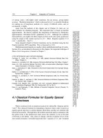
Figure 4.1.1. Quadrature formulas with equally spaced abscissas compute the integral of a function
between x
0
and x
N +1
. Closed formulas evaluate the function on the boundary points, while open
formulas refrain from doing so (useful if the evaluation algorithm breaks down on the boundary points).
midpoint rule,” equation 4.1.19, see §4.2), the classical formulas are almost entirely
useless. They are museum pieces, but beautiful ones.
Some notation: We have a sequence of abscissas, denoted x
0
,x
1
,...,x
N
,
x
N+1
which are spaced apart by a constant step h,
x
i
= x
0
+ ih i =0,1,...,N+1 (4.1.1)
A function f(x) has known values at the x
i
’s,
f (x

i
) ≡ f
i
(4.1.2)
We want to integrate the function f(x) between a lower limit a and an upper limit
b,whereaand b are each equal to one or the other of the x
i
’s. An integration
formula that uses the value of the function at the endpoints, f(a) or f(b), is called
a closed formula. Occasionally, we want to integrate a function whose value at one
or both endpoints is difficult to compute (e.g., the computation of f goes to a limit
of zero over zero there, or worse yet has an integrable singularity there). In this
case we want an open formula, which estimates the integral using only x
i
’s strictly
between a and b (see Figure 4.1.1).
The basic building blocks of the classical formulas are rules for integrating a
function over a small number of intervals. As that number increases, we can find
rules that are exact for polynomials of increasingly high order. (Keep in mind that
higher order does not always imply higher accuracy in real cases.) A sequence of
such closed formulas is now given.
Closed Newton-Cotes Formulas
Trapezoidal rule:

x
2
x
1
f(x)dx = h


1
2
f
1
+
1
2
f
2

+ O(h
3
f

)(4.1.3)
Here the error term O()signifies that the true answer differs from the estimate by
an amount that is the product of some numerical coefficient times h
3
times the value
132
Chapter 4. Integration of Functions
Sample page from NUMERICAL RECIPES IN C: THE ART OF SCIENTIFIC COMPUTING (ISBN 0-521-43108-5)
Copyright (C) 1988-1992 by Cambridge University Press.Programs Copyright (C) 1988-1992 by Numerical Recipes Software.
Permission is granted for internet users to make one paper copy for their own personal use. Further reproduction, or any copying of machine-
readable files (including this one) to any servercomputer, is strictly prohibited. To order Numerical Recipes books,diskettes, or CDROMs
visit website or call 1-800-872-7423 (North America only),or send email to (outside North America).
of the function’s second derivative somewhere in the interval of integration. The
coefficient is knowable, and it can be found in all the standard references on this
subject. The point at which the second derivative is to be evaluated is, however,
unknowable. If we knew it, we could evaluate the function there and have a higher-

order method! Since the product of a knowable and an unknowable is unknowable,
we will streamline our formulas and write only O(), instead of the coefficient.
Equation (4.1.3) is a two-point formula (x
1
and x
2
). It is exact for polynomials
up to and including degree 1, i.e., f(x)=x. One anticipates that there is a
three-point formula exact up to polynomials of degree 2. Thisis true; moreover, by a
cancellation of coefficients due to left-rightsymmetry of the formula, the three-point
formula is exact for polynomials up to and including degree 3, i.e., f(x)=x
3
:
Simpson’s rule:

x
3
x
1
f(x)dx = h

1
3
f
1
+
4
3
f
2

+
1
3
f
3

+ O(h
5
f
(4)
)(4.1.4)
Here f
(4)
means the fourth derivative of the function f evaluated at an unknown
place in the interval. Note also that the formula gives the integral over an interval
of size 2h, so the coefficients add up to 2.
There is no lucky cancellation in the four-point formula, so it is also exact for
polynomials up to and including degree 3.
Simpson’s
3
8
rule:

x
4
x
1
f(x)dx = h

3

8
f
1
+
9
8
f
2
+
9
8
f
3
+
3
8
f
4

+ O(h
5
f
(4)
)(4.1.5)
The five-point formula again benefits from a cancellation:
Bode’s rule:

x
5
x

1
f(x)dx = h

14
45
f
1
+
64
45
f
2
+
24
45
f
3
+
64
45
f
4
+
14
45
f
5

+ O(h
7

f
(6)
)(4.1.6)
This is exact for polynomials up to and including degree 5.
At this point the formulas stop being named after famous personages, so we
will not go any further. Consult
[1]
for additional formulas in the sequence.
Extrapolative Formulas for a Single Interval
We are going to depart from historical practice for a moment. Many texts
would give, at this point, a sequence of “Newton-Cotes Formulas of Open Type.”
Here is an example:

x
5
x
0
f(x)dx = h

55
24
f
1
+
5
24
f
2
+
5

24
f
3
+
55
24
f
4

+ O(h
5
f
(4)
)
4.1 Classical Formulas for Equally Spaced Abscissas
133
Sample page from NUMERICAL RECIPES IN C: THE ART OF SCIENTIFIC COMPUTING (ISBN 0-521-43108-5)
Copyright (C) 1988-1992 by Cambridge University Press.Programs Copyright (C) 1988-1992 by Numerical Recipes Software.
Permission is granted for internet users to make one paper copy for their own personal use. Further reproduction, or any copying of machine-
readable files (including this one) to any servercomputer, is strictly prohibited. To order Numerical Recipes books,diskettes, or CDROMs
visit website or call 1-800-872-7423 (North America only),or send email to (outside North America).
Notice that the integral from a = x
0
to b = x
5
is estimated, using only the interior
points x
1
,x
2

,x
3
,x
4
. In our opinion, formulas of this type are not useful for the
reasons that (i) they cannot usefully be strung together to get “extended” rules, as we
are about to do with the closed formulas, and (ii) for all other possible uses they are
dominated by the Gaussian integration formulas which we will introduce in §4.5.
Instead of the Newton-Cotes open formulas, let us set out the formulas for
estimating the integral in the single interval from x
0
to x
1
, using values of the
function f at x
1
,x
2
,.... These will be useful building blocks for the “extended”
open formulas.

x
1
x
0
f(x)dx = h[f
1
]+O(h
2
f


)(4.1.7)

x
1
x
0
f(x)dx = h

3
2
f
1
−
1
2
f
2

+ O(h
3
f

)(4.1.8)

x
1
x
0
f(x)dx = h


23
12
f
1
−
16
12
f
2
+
5
12
f
3

+ O(h
4
f
(3)
)(4.1.9)

x
1
x
0
f(x)dx = h

55
24

f
1
−
59
24
f
2
+
37
24
f
3
−
9
24
f
4

+ O(h
5
f
(4)
)(4.1.10)
Perhaps a word here would be in order about how formulas like the above can
be derived. There are elegant ways, but the most straightforwardis to write down the
basic form of the formula, replacing the numerical coefficients with unknowns, say
p, q, r, s. Without loss of generality take x
0
=0and x
1

=1,soh=1. Substitutein
turn for f(x) (and for f
1
,f
2
,f
3
,f
4
) the functions f(x)=1,f(x)=x,f(x)=x
2
,
and f(x)=x
3
. Doing the integral in each case reduces the left-hand side to a
number, and the right-hand side to a linear equation for the unknowns p, q, r, s.
Solving the four equations produced in this way gives the coefficients.
Extended Formulas (Closed)
If we use equation (4.1.3) N − 1 times, to do the integration in the intervals
(x
1
,x
2
),(x
2
,x
3
),...,(x
N−1
,x

N
), and then add the results,we obtain an “extended”
or “composite” formula for the integral from x
1
to x
N
.
Extended trapezoidal rule:

x
N
x
1
f(x)dx = h

1
2
f
1
+ f
2
+ f
3
+
···+f
N−1
+
1
2
f

N

+O

(b−a)
3
f

N
2

(4.1.11)
Here we have written the error estimate in terms of the interval b − a and the number
of points N instead of in terms of h. This is clearer, since one is usually holding
a and b fixed and wanting to know (e.g.) how much the error will be decreased
134
Chapter 4. Integration of Functions
Sample page from NUMERICAL RECIPES IN C: THE ART OF SCIENTIFIC COMPUTING (ISBN 0-521-43108-5)
Copyright (C) 1988-1992 by Cambridge University Press.Programs Copyright (C) 1988-1992 by Numerical Recipes Software.
Permission is granted for internet users to make one paper copy for their own personal use. Further reproduction, or any copying of machine-
readable files (including this one) to any servercomputer, is strictly prohibited. To order Numerical Recipes books,diskettes, or CDROMs
visit website or call 1-800-872-7423 (North America only),or send email to (outside North America).
by taking twice as many steps (in this case, it is by a factor of 4). In subsequent
equations we will show only the scaling of the error term with the number of steps.
For reasons that will not become clear until §4.2, equation (4.1.11) is in fact
the most important equation in this section, the basis for most practical quadrature
schemes.
The extended formula of order 1/N
3
is:


x
N
x
1
f(x)dx = h

5
12
f
1
+
13
12
f
2
+ f
3
+ f
4
+
···+f
N−2
+
13
12
f
N −1
+
5

12
f
N

+ O

1
N
3

(4.1.12)
(We will see in a moment where this comes from.)
If we apply equation (4.1.4) to successive, nonoverlapping pairs of intervals,
we get the extended Simpson’s rule:

x
N
x
1
f(x)dx = h

1
3
f
1
+
4
3
f
2

+
2
3
f
3
+
4
3
f
4
+
···+
2
3
f
N−2
+
4
3
f
N−1
+
1
3
f
N

+O

1

N
4

(4.1.13)
Notice that the 2/3, 4/3 alternation continues throughout the interior of the evalu-
ation. Many people believe that the wobbling alternation somehow contains deep
information about the integral of their function that is not apparent to mortal eyes.
In fact, the alternation is an artifact of using the building block (4.1.4). Another
extended formula with the same order as Simpson’s rule is

x
N
x
1
f(x)dx = h

3
8
f
1
+
7
6
f
2
+
23
24
f
3

+ f
4
+ f
5
+
···+f
N−4
+f
N−3
+
23
24
f
N −2
+
7
6
f
N −1
+
3
8
f
N

+ O

1
N
4


(4.1.14)
This equation is constructed by fitting cubic polynomials through successive groups
of four points; we defer details to §18.3, where a similar technique is used in the
solution of integral equations. We can, however, tell you where equation (4.1.12)
came from. It is Simpson’s extended rule, averaged with a modified version of
itself in which the first and last step are done with the trapezoidal rule (4.1.3). The
trapezoidal step is two orders lower than Simpson’s rule; however, its contribution
to the integral goes down as an additional power of N (since it is used only twice,
not N times). This makes the resulting formula of degree one less than Simpson.