Moving parabolic approximation model of point clouds and its application
Bạn đang xem bản rút gọn của tài liệu. Xem và tải ngay bản đầy đủ của tài liệu tại đây (930.85 KB, 7 trang )
VNU Journal of Science, Natural Sciences and Technology 24 (2008) 179-185
Moving parabolic approximation model
of point clouds and its application
Zhouwang Yang1, Tae-wan Kim2*
1
Department of Naval Architecture and Ocean Engineering
Seoul National University, Seoul 151-744, Korea
2
Department of Naval Architecture and Ocean Engineering
and Research Institute of Marine Systems Engineering,
Seoul National University, Seoul 151-744, Korea
Received 31 October 2007
Abstract. We propose the moving parabolic approximation (MPA) model to reconstruct an
improved point-based surface implied by an unorganized point cloud, while also estimating the
differential properties of the underlying surface. We present examples which show that our
reconstructions of the surface, and estimates of normal and curvature information, are accurate for
precise point clouds and robust in the presence of noise. As an application, our proposed model is
used to generate triangular meshes approximating point clouds.
1. Introduction*
geometric modeling [4]. The point-based
representation of a surface should be as
compact as possible, meaning that it is neither
noisy nor redundant. It is therefore important to
develop algorithms which generate compact
point sets from nonuniform and noisy input, so
as effectively to reconstruct the underlying
surfaces. It should also be possible to recover
the intrinsic geometric properties of the
underlying surfaces as precisely as possible
from point clouds.
Differential quantities such as normals,
principal curvatures, and principal directions of
curvature can be used for a variety of tasks in
computer graphics, computer vision, computeraided
design,
geometric
modeling,
computational geometry, and industrial and
biomedical engineering. A number of methods
for curvature estimation have been published by
Acquiring large amounts of point data from
real objects has become more convenient
because of modern sensing technologies and
digital scanning devices. However, the data
acquired is usually distorted by noise, arising
out of physical measurement processes, and by
the limitations of the acquisition technologies.
Even so, it is possible to obtain the smooth
underlying shapes which are implied by an
unstructured point cloud. Consequently,
techniques of reconstructing models from noisy
data sets are receiving increasing attention.
Point-based surfaces [1-3] have recently
become an appealing shape representation in
computer graphics and can be used for
_______
*
Corresponding author. Email:
179
180 Zhouwang Yang, Tae-wan Kim / VNU Journal of Science, Natural Sciences and Technology 24 (2008) 179-185
various communities, but mostly for manifold
representations of the surface such as
polyhedral meshes, or oriented data sets such as
points paired with normals. We would like to
recover the differential properties of an
underlying
surface
directly
from
an
unstructured point cloud, even though it may be
nonuniform and noisy. Our approach, motivated
by some recent work of Levin [2], is based on
local maps of differential geometry [5] and
practical algorithms in optimization theory [6]. The
main contribution of this work is a scheme to
generate a point-based reconstruction of an
unorganized point cloud and simultaneously to
estimate the differential properties of the
underlying surface. As an application, we will used
the proposed technique to reconstruct triangular
meshes approximating given point clouds.
2. Moving parabolic approximation
Recently, there has been increasing interest
expressed in surface modeling using
unorganized data points. A powerful approach
is the use of the moving least-squares (MLS)
technique [2] for modeling point-based surfaces
[1]. One of the main strengths of MLS
projection is its ability to handle noisy data. We
extend the MLS technique to a moving
parabolic approximation (MPA), which is a
model of a second-order projection. The MPA
model is naturally framed as an optimization
problem based on the following proposition:
Proposition 1: At every point p on a
surface S , there exists an osculating paraboloid
Sp* such that the normal curvature of Sp* is
identical to that of S at p for any tangent vector.
due to noise. We first define a neighborhood of the
given point cloud in the form:
n
B( r ) = ∪ {x ∈ R 3
x − pj ≤ r }
(1)
j =1
With an assumption
r ≥ max min p j1 − p j 2
j1
(2)
j 2≠ j 1
we ensure that the neighborhood B(r) contains
the underlying surface as well as the
approximation that we are going to construct. A
number of points in this neighborhood are
chosen for reference, called reference points,
which will be projected on to the underlying
surface using MPA models.
Let x ∈ B(r) be a reference point in the
close neighborhood of the given data points.
The foot-point of x on the underlying surface S
is denoted as
o x = x + ζn,
(3)
where n is the unit normal to S, and ζ is the
signed distance from x to ox along n. We aim to
compute the foot-point ox and the differential
quantities at the foot-point. Let {t1(n), t2(n)}be
the perpendicular unit basis vectors of the
tangent plane, so that {ox; t1, t2, n}forms a local
orthogonal coordinate system. Writing qj = pj −
x, we formulate the moving parabolic
approximation model as a constrained
optimization:
n
minf (n, ζ,a,b,c ) =
∑ [q
T
j
n−ζ
j =1
−
2
2
1
− a (qTj t1 ) + 2b (qTj t1 )(qTj t2 ) + c (qTj t2 ) ] 2 e
2
(
)
q j −ζn
p
2
2
(4)
where (n,ζ,a,b,c) are decision variables and ρ is
a scale parameter.
2.1. MPA model
n
Suppose that a given set of data points {p j }j =1
is noisy sampling of an underlying surface S.
Generally, pj will not lie on the underlying shape S
Once the optimum solution (n*,ζ*,a*,b*,c*)of
the MPA model of Equation (4) has been
obtained, we can recover the differential
quantities of the underlying surface S at the
181
Zhouwang Yang, Tae-wan Kim / VNU Journal of Science, Natural Sciences and Technology 24 (2008) 179-185
foot-point ox = x + ζ*n*, including the principal
curvatures and the principal directions of
curvature. An osculating paraboloid of the
underlying surface at ox can then be represented
by the parametric expression
T
1
S * (u , v ) = u , v, a *u 2 + 2b *uv + c * v 2 ,
2
(
)
(5)
The principal directions e*min and e*max are
always orthogonal to each other except at the
umbilical
points.
At
an
umbilic,
*
*
κ min = κ max holds, and the surface is locally part
of sphere with a radius of 1/H*. In the special
case where the identical principal curvatures
vanish, the surface becomes locally flat.
in the local coordinate system {ox; t*1 , t*2 ,n*}.
The first fundamental form of S*(u,v) is given by
*
2
2
I = Edu + 2Fdudv + Gdv ,
(6)
where E =1, F =0 and G =1 at the foot-point ox.
The second form of S*(u,v) is given by
II * = Ldu 2 + 2Mdudv + Ndv 2 ,
(7)
where L = a*, M = b* and N = c*. The mean
curvature H* and the Gaussian curvature K* can
now be calculated as follows:
H* =
LG − 2 MF + NE a * + c *
=
, (8)
2
2 EG − F 2
(
)
2
LN − M 2
K =
= a *c * − b* .
2
EG − F
*
From this calculation and Proposition 1,
we obtain the minimum and maximum
principal curvatures of the underlying surface
S at ox:
κ* = H * − H * 2 − K * ,
min
(9)
*
*
*2
*
κ
= H + H −K .
max
and the corresponding principal directions of
curvature in the tangent plane:
e*min = t*1 ,e*max = t*2 ,if κ*min = a* ≤ c* = κ*max ;
e*min =
b* t1* + ( κ*min −a* ) t*2
* 2
2
,
(κ*min −a ) + b*
(κ*max −c* ) t1* +b*t*2
*
emax =
, otherwise.
2
(κ*max −c* ) + b*
2
(10)
2.2. Implementation and examples
The MPA model of Equation (4) is a
constrained optimization problem. We solve
this constrained optimization by a practical
algorithm based on Lagrange-Newton method
[6]. We implement our MPA approach and
perform it on a number of point clouds.
The moving parabolic approximation model
was tested on several different shapes of
surface. Each shape is a graph of a bivariate
function z(x,y) defined over [−1,1] × [−1,1] and
evaluated using a 41 × 41 grid.
(xl , y k ) = (− 1 + l / 20,−1 + k / 20 ), k= 0,…,40,
to determine a set of clean points that lie on the
graph:
Pclean =
{(x ,y ,z (x ,y ))
T
l
k
l
k
}
l,k = 0,..., 40
In order to verify the stability of the
algorithm, we generated a point cloud P noise by
adding Gaussian noise with a magnitude of 1%
of the overall cloud dimension to clean data.
The four test surfaces were a sphere
(x, y, z )T
(x, y, z )T
(x, y, z )T
(
= (x, y ,
= x, y , 4 − x 2 − y 2
(
2 − x2
),
a cylinder
a
paraboloid
),
T
T
)
(x, y, z ) = (x, y, x
T
= x, y, x 2 + y 2 ,
T
and
2
)
2 T
a
hyperboloid
− y . The
estimated curvature information obtained from
MPA model was compared with the exact
curvatures in each case. We measured the
182 Zhouwang Yang, Tae-wan Kim / VNU Journal of Science, Natural Sciences and Technology 24 (2008) 179-185
difference in terms of root-mean-square (RMS)
error, which we define as
2
1 m
valiest − valiex ,
∑
m i =1
(
Err =
)
(11)
where valiest represents one of the estimated
values
κest
min ,
est
k max
, Hest or Kest, and
valiex represents one of the exact values
ex
ex
κex
or Kex. Table I summarizes
min , κ max , H
the RMS errors that occurred in the
estimation of principal, mean and Gaussian
curvatures. From which, we observe that
our MPA algorithm can obtain robust and
accurate estimates in the presence of noise
as well as for clean data.
We also applied the MPA algorithm to the
scanning data set of a mouse which contains
36036 points, and presented the point-based
reconstruction and the estimates of curvature in
Figure 1. The results show the confidence of
our MPA method for reverse engineering
applications.
Table 1. RMS errors in curvature estimation for the
test surfaces
Example
Sphere
(clean data)
(with 1% noise)
Cylinder
(clean data)
(with 1% noise)
Paraboloid
(clean data)
(with 1% noise)
Hyperboloid
(clean data)
(with 1% noise)
Err ( κ min ) Err ( κ max ) Err (H )
Fig. 1. Applying the MPA algorithm
to the Mouse model.
Err (K )
0.0028
0.0412
0.0014
0.0264
0.0019
0.0233
0.0019
0.0238
0.0038
0.0747
3.5e-07
0.0281
0.0019
0.0446
2.5e07
0.0215
0.0144
0.0957
0.0188
0.1075
0.0158
0.0885
0.0287
0.1828
0.0117
0.1278
0.0017
0.1297
0.0028
0.0684
0.0138
0.1505
3. Mesh reconstruction
As an application, our MPA model is used
to generate a triangular mesh that approximates
the underlying surface of given point cloud.
Our method of mesh reconstruction from point
clouds by moving parabolic approximation can
be outlined in the following scheme.
1.
A rough initial mesh M(0) = (V(0), E(0)) is
constructed from given point cloud
n
P = {p j }j =1 ⊂ ℝ 3 . Let VNew:= V(0) be the
initial set of new inserting vertices.
Zhouwang Yang, Tae-wan Kim / VNU Journal of Science, Natural Sciences and Technology 24 (2008) 179-185
2.
Repeatedly apply the steps of curvaturebased refinement (a-b-c) until the
approximation error is within a predefined
tolerance or the maximal number of times
is reached:
a. For each vN ∈ VNew, we project it on to
the underlying surface of the point cloud
P using the MPA algorithm, and get the
estimate of mean curvature vector KP(v)
at the projection v = MPA(vN). After
projection, the set of potential vertices is
denoted by
{
V Potential = v = MPA ( vN ) ∀vN ∈ V New and K P (v) 〉 σ
3.
183
connections for those new inserting
vertices.
Output the resulting mesh M = (V, E) as
the final approximation to the input point
cloud P.
Figures 2 to 4 show the meshes
reconstructed from given point clouds using our
MPA algorithm.
}
b. Calculate the mean curvature normal
KM(v) via the differential geometry
operator [7], and define
V Active =
{v
∈V Potential KM ( v) − KP (v) 〉ε KP (v)
}
as the collection of active vertices.
c. Insert a new vertex at the midpoint of
every edge adjacent to any v ∉ V Active ,
and
then
renew
v + vi
New
N
Active
V
= v =
|∀ v ∈ V
2
and vvi ∈ E }. The approximating mesh
is updated by adding the topological
{
}
Fig. 2. Mesh reconstruction for the Knot model
(a) the data points (b) the initial mesh
184 Zhouwang Yang, Tae-wan Kim / VNU Journal of Science, Natural Sciences and Technology 24 (2008) 179-185
(c) the mesh after one iteration (d) the mesh after two iterations
Fig. 3. Mesh reconstruction for the Horse model.
(a) the data points
(c) the mesh after one iteration
(b) the initial mesh
(d) the mesh after two itenrations
Fig. 4. Mesh reconstruction for the Sculpture model.
Zhouwang Yang, Tae-wan Kim / VNU Journal of Science, Natural Sciences and Technology 24 (2008) 179-185
4. Conclusion
We have shown how to construct an
improved point-based representation from a
point cloud, at the same time as computing the
normals and curvatures of the underlying shape.
Our algorithm is based on optimization theory
and works robustly in the presence of noise,
while yielding accurate estimates for clean data.
The effectiveness of the algorithm has been
demonstrated in the reconstruction of point
clouds obtained by sampling several different
surfaces, including a sphere, a cylinder, a
paraboloid and a hyperboloid.
As an application, we use the MPA
algorithm to construct a triangular mesh
approximating the underlying surface of a given
point cloud. We expect that our MPA method
will find further applications in many
operations on point-based surfaces, such as
smoothing,
simplification,
segmentation,
feature extraction, global registration.
Acknowledgments. This work was supported
by grant No. R01-2005-000-11257-0 from the
Basic Research Program of the Korea Science
and Engineering Foundation, and in part by
Seoul R&BD Program. We would like to thank
185
the INUS Technology Inc for providing
scanning data points of the Mouse model.
References
[1] A. Alexa, J. Behr, D. Cohen-Or, S. Fleishman, D.
Levin, C. Silva, “Point set surfaces’, In
Proceedings of IEEE Visualization (2001) 21,.
[2] D.
Levin,
“Mesh-independent
surface
interpolation”, In Brunnett, B. Hamann, and H.
Mueller, editors, Geometric Modeling for
Scientific Visualization, Springer-Verlag, (2003)
37.
[3] N. Amenta, Y.J. Kil, “Defining point-set
surfaces”, In Proceedings of ACM SIGGRAPH
(2004) 264.
[4] M. Pauly, R. Keiser, L.P. Kobbelt, M. Gross,
“Shape modeling with point-sampled geometry”,
In Proceedings of ACM SIGGRAPH (2003) 6.
[5] P.M. do Carmo, “Differential Geometry of Curves
and Surfaces”, Prentice-Hall, 1987.
[6] R. Fletcher,
“Practical
Methods
of
Optimization”, John Wiley & Sons, 2nd edition,
1987.
[7] M. Meyer, M. Desbrun, P. Schroder, A.H. Barr,
“Discrete differential-geometry operators for
triangulated 2-manifolds”, In H.C. Hege and K.
Polthier, editors, Visualization and Mathematics
III, Springer-Verlag, (2003) 35.