Logit models for forecasting nationwide intercity travel demand in the united states
Bạn đang xem bản rút gọn của tài liệu. Xem và tải ngay bản đầy đủ của tài liệu tại đây (607.67 KB, 12 trang )
Logit Models for Forecasting
Nationwide Intercity Travel Demand
in the United States
Senanu Ashiabor, Hojong Baik, and Antonio Trani
There are 3,091 counties in TSAM serving as the zones of travel
activity in the continental United States. The trip-generation output is
made up of two 3091 vectors: one for attractions and the other for productions for each county. Trip distribution fills up the cells between
the vectors, creating a person-trip interchange table of demand
between the two counties. Mode choice splits the demand between
each county by mode of transportation. The mode choice model
in TSAM and this paper estimates both the demand by mode between
counties and the demand flows in the airport network associated with
the counties. This is achieved by embedding an airport choice model
in the mode choice model. Hence the model is both a mode choice and
a partial trip assignment model. The framework for the process is
shown in Figure 1. The modes of transportation considered in the
TSAM model are commercial airline, automobile, SATS, and train.
However, the focus in this paper is on the baseline model, which has
only automobile and commercial airline modes. The trip assignment
in TSAM involves converting the airport-to-airport person trips into
aircraft operations, generating flights by using a time-of-day profile,
and loading the flights on the National Airspace System to estimate
the impact of aircraft operations in the system. The complete travel
demand model is fully documented elsewhere (1–3).
NASA is using TSAM to forecast future airport demands and
assist the Joint Program Development Office (JPDO) in planning
the next-generation air transportation system. NASA is also using
TSAM to study demand for supersonic aircraft, tilt rotors, and short
take-off and landing aircraft. This shows that the model is relevant
and the output is critical to policy makers.
This paper presents a family of logit models that have been developed since the SATS program to estimate intercity travel demand in
the United States.
Nested and mixed logit models were developed to study national-level
intercity transportation in the United States. The models were used to
estimate the market share of automobile and commercial air transportation of 3,091 counties and 443 commercial service airports in the United
States. Models were calibrated with the use of the 1995 American Travel
Survey. Separate models were developed for business and nonbusiness
trip purposes. The explanatory variables used in the utility functions of
the models were travel time, travel cost, and traveler’s household income.
Given an input county-to-county trip demand table, the models were used
to estimate county-to-county travel demand by automobile and commercial airline between all counties and commercial-service airports in the
United States. The model has been integrated into a computer software
framework called the transportation systems analysis model that estimates nationwide intercity travel demand in the United States.
In 2000, the National Aeronautics and Space Administration (NASA)
proposed to Congress the development of a small aircraft transportation system (SATS) to harness the potential of the nation’s vast
network of underutilized airports. As part of the SATS program,
NASA assigned the Air Transportation Systems Laboratory at Virginia
Polytechnic Institute and State University (Virginia Tech) the task
of developing a transportation systems analysis model to estimate the
demand for SATS vehicles. Virginia Tech used the classical four-step
transportation planning procedure to develop a framework called the
transportation systems analysis model (TSAM) to estimate demand
for intercity trips when a novel mode of transportation such as SATS
is introduced. The four-step planning model is a sequential demand
forecasting model made up of trip generation, trip distribution, mode
choice, and trip assignment.
Trip generation estimates the number of trips produced and attracted
to each zone of activity by trip purpose. Trip distribution estimates
origin–destination flows, thereby linking trip ends from the trip
generation to form trip interchanges between zones. Mode choice
estimates the percentage of travelers by using each mode of transportation between each origin–destination pair. Trip assignment loads the
origin–destination flows of each mode on specific routes through the
respective transportation networks.
LITERATURE REVIEW
Review of Disaggregate Nationwide
Travel Demand Models
Between 1976 and 1990, four major attempts were made to develop
disaggregate national-level intercity mode choice models in the
United States. All the models used versions of National Travel Surveys (NTS) conducted by the Bureau of the Census and the Bureau
of Transportation Statistics (BTS). The first was a multinomial logit
model by Stopher and Prashker in 1976, which used the 1972 NTS (4).
Grayson developed a multinomial logit model by using the 1977 version of the NTS (5). Morrison and Winston were the first to apply a
nested logit model (6). They used the log-sum variable to hierarchically nest three models: decision to rent a car, destination choice, and
mode choice. Later, Koppelman extended Morrison’s approach to
S. Ashiabor, 301S Patton Hall, and H. Baik and A. Trani, 200 Patton Hall, Department of Civil and Environmental Engineering, Virginia Polytechnic Institute and
State University, Blacksburg, VA 24061. Corresponding author: S. Ashiabor,
Transportation Research Record: Journal of the Transportation Research Board,
No. 2007, Transportation Research Board of the National Academies, Washington,
D.C., 2007, pp. 1–12.
DOI: 10.3141/2007-01
1
2
Transportation Research Record 2007
FIGURE 1
Multistep illustration of intercity transportation modeling process.
hierarchically nest a set of trip frequency, trip destination, mode
choice, and fare class choice models by using log-sum values and the
1997 NTS database (7). All the models had automobile, air, bus, and
rail as their set of transportation models. Details of the four models
and the variables in their utility function are summarized in Table 1.
Traveler mode choice information was extracted from the NTS
surveys. However, these surveys did not contain information on levelof-service variables. Thus the authors developed synthetic travel
time and cost data from published fare and schedule guides, such as
the official airline, railroad, and bus guides. They all restricted their
analysis to trips starting and ending in metropolitan statistical areas
(MSAs). The main reason for this is that trips in the surveys are
identified only by state and whether they are in an MSA. It is very
difficult to estimate travel times and costs for any trip originating or
ending in non-MSA areas given the size of most states.
All model coefficients had the expected signs; however, in the
case of the two multinomial logit models, the elasticity estimates
were counterintuitive. The authors attributed model weaknesses to
the poor quality of the NTS data and to tenuous assumptions made in
derivation of the level of service variables. Koppelman et al. also
noted that a high level of geographic aggregation, poor information
on the choice set, and lack of service variables are additional limitations in the development of robust models (8). The issue of elasticity
estimates of multinomial logit models and their appropriateness for
forecasting and sensitivity analysis are discussed later.
The major constraints in developing credible models are related
more to the NTS databases than the modeling techniques. The two
major issues are the restriction of the minimum level of geographical detail to MSA and the absence of information related to airports
and access and egress distances to airports and terminals. Koppel-
Ashiabor, Baik, and Trani
TABLE 1
3
Major National-Level Intercity Travel Demand Models for the United States
Model Type
Data and Scope
Stopher and
Prashker
(1976)
Multinomial
logit
Alan Grayson
(1982)
Multinomial
logit
Morrison and
Winston
(1985)
Nested logit
Koppelman
(1990)
Nested logit
Mode choice
model in
TSAM
Nested logit and
mixed logit
models
Database: 1972 NTS
Scope: trips that start and end
in MSAs
2,085 records from database
Database: 1977 NTS
Scope: trips that start and end
in MSAs
Selected observations from
database
Database: 1977 NTS
Scope: trips that start and end
in MSAs
4,218 records from database
Database: 1977 NTS
Scope: trips that start and end
in MSAs
Selected observations from
database
Database: 1995 American
Travel Survey
Scope: all trips regardless of
origin or destination type
402,295 records from database
Modes of
Transportation
Variables in Utility Function
Market
Segmentation
Automobile,
commercial air,
bus, rail
Relative time, relative distance,
relative cost, relative
access–egress distance,
departure frequency
Trip purpose
(business–
nonbusiness)
Automobile,
commercial air,
bus, rail
Travel time, travel cost, access
time, and departure
frequency
Trip purpose
(business–
nonbusiness)
Automobile,
commercial air,
bus, rail
Travel time, cost, party size,
average time between
departures
Trip purpose
(business–
nonbusiness)
Automobile,
commercial air,
bus, rail
Travel time, cost, departure
frequency, distance between
city pairs, household income
Trip purpose
(business–
nonbusiness)
Automobile,
commercial air,
train, SATS
Travel time, travel cost,
household income, region
type
Trip purpose
(business–
nonbusiness)
Household income
MSA = metropolitan statistical area.
man and Hirsh expounded on the data requirements for researchers
and practitioners to develop accurate and useful intercity travel
demand models (9). However, there appears to be no attempt by
any of the key federal agencies (Census Bureau or BTS) to collect
such data.
The mode choice models presented in this paper extend the work
of national-level intercity travel demand modeling in three dimensions. The spatial extent of the model is extended to include non-MSA
areas so the model can be applied nationally. Second, an airport
choice model is implemented with the mode choice so that the model
can estimate market share of the airport network to make it more useful to policy makers. Third, level-of-service variables are aggregated
at the county level, giving the model a broader scope since county
socioeconomic variable forecasts exists at this level. This is the first
national level, intercity, multimode choice model to model both mode
choice and airport choice at the county level in the United States.
Review of Logit Models
McFadden (10) developed the multinomial logit model based on
Luce’s (11) axiom of independence of irrelevant alternatives (IIA).
The model assumed an underlying Gumbel distribution and a random
sample that is independent and identically distributed (IID), implying that the alternatives being considered are independent of each
other and have the same variance. The multinomial logit probability
has the form shown in Equation 1:
P (i ) =
eVi
∑
J
j =1
e
Vj
(1)
It is clear from Equation 1 that for any two alternatives k and l,
the ratio of their probabilities
P ( k ) e Vk
=
P ( l ) e Vl
is independent of any other alternatives in the model. The constant
nature of this ratio regardless of the presence of other alternatives,
however, produces unrealistic substitution patterns associated with
the IIA property.
Ben-Akiva and Lerman used the now-famous red bus–blue bus
problem to show how IIA produces wrong estimates when a new
mode with similar characteristics is introduced into the choice set
(12). IIA also affects cross-elasticity estimates of the model. Consider
the impact of the change in an attribute of an alternative j on the probability Pni of all other alternatives in the model. The change in Pni with
respect to a change in the attribute of j is given as Equation 2 (13):
EiZnj = −β z Z nj Pnj
(2)
where Znj is the attribute of alternative j faced by individual n, and βz
is its coefficient. Since the cross elasticity is the same for all i, the
implication is that an improvement in any one alternative reduces the
probabilities of all the other alternatives by the same amount (that is,
EiZnj is fixed for all i). This means that if a model has three alternatives,
and a policy is implemented to improve one mode, the multinomial
logit model will draw the same percentage from the remaining modes.
Such a result is unrealistic, and it is not surprising that elasticity estimates from Grayson’s (5) and Stopher’s (4) multinomial logit models did not yield intuitive estimates. The multinomial logit model is
analytically tractable because of its closed form; however, the IIA
property renders it unsuitable for policy studies that seek to investigate the impact of improving or introducing new alternatives. To
develop more flexible empirical models, there has been a shift toward
relaxing the independence or identical distribution assumptions while
maintaining the analytically closed form of the model.
The first attempt was the nested logit model that relaxes the independence assumption by grouping similar alternatives into nests
4
Transportation Research Record 2007
(14, 15). Other models that relax the independence assumption are
cross-nested logits (16, 17 ), ordered generalized extreme value
models (18, 19), Chu’s paired combinatorial logit (20), and Wen and
Koppelman’s generalized nested logit (21). McFadden specified a
generalized extreme value (GEV) joint distribution that allows for
any form of correlation that is an overarching framework over all
these models, including the logit model.
A detailed discussion on GEV models is available from Train (13)
and Ben-Akiva and Lerman (12). By using the GEV framework that the
nested logit model has choice probability of the form in Equation 3,
P (i ) =
Yi Gi
=
G
⎛
⎞
YiYi(1/ λl )−1 ⎜ ∑ Y j1/ λl ⎟
⎝ j∈Bk
⎠
⎛
⎞
∑ l =1 ⎜⎝ ∑ Yj1/ λl ⎟⎠
λ k −1
λl
=
⎛
⎞
Yi1/ λ k ⎜ ∑ Y j1/ λl ⎟
⎝ j∈Bk
⎠
K
λ k −1
⎛
⎞
∑ l =1 ⎜⎝ ∑ Yj1/ λl ⎟⎠
λl
j ∈Bk
substituuting eVi
Vi
=
)
(e ) (∑ (e )
λk
1/ λ k
Vj
j ∈Bk
⎛
V
∑ l =1 ⎜⎝ ∑ e j
K
j ∈Bk
( )
1/ λ l
λ k −1
λl
⎞
⎟⎠
=
eVi / λ k
(∑
j ∈Bk
e
V j / λl
)
⎛
V /λ ⎞
∑ l =1 ⎜⎝ ∑ e j l ⎟⎠
λ k −1
λl
(3)
K
j ∈Bk
where Yi = evi and G is a function with well defined properties that
depends on Yi and can be denoted G = G(Y1, . . . , YI). Gi is the derivative Gi = δG/δYi [see Train(13), pp. 97–100, for complete derivation;
j ∈ Bk implies alternative j belongs to nest Bk.
Clearly, for any two alternatives i ∈ Bk and m ∈ Bl in different nests,
eVi λ k
P (i )
=
P ( m ) eVm λl
(∑
(∑
j ∈Bk
e
Vj λk
e
j ∈B
l
V j λl
)
)
Unj = α n x nj + ⑀ nj
(5)
⎛ e αxni
Pni = ∫ ⎜
⎜⎝ ∑ e αxnj
j
⎞
⎟ f ( α ) dα
⎟⎠
(6)
The researcher specifies a distribution for the coefficients αn and
estimates the parameters of the distributions (say, mean and variance).
The utility function takes the form of a weighted average of the logit
formula estimated at different values of α with weights given by the
density f(α), as shown in Equation 6. Common distributions used in
practice are the normal, lognormal, triangular, and uniform.
Error-Components Mixed Logit
λ k −1
λ l −1
In all logit models considered so far, the utility takes the form Unj =
αxnj + ⑀nj, where xnj is a vector of attributes that relate to the individual n and alternatives j. The error term ⑀nj is IID extreme value. The
coefficient α is fixed for each attribute xnj. In the random-coefficients
mixed logit in Equation 5, the vector of coefficients αn is not fixed
but rather varies over individuals n with a density f(α).
The decision maker knows the complete value of their utility in
the form of the values of αn and ⑀nj and selects the alternative with
the highest utility; however, the researcher observes only the choice
and the xnj but not coefficients αn and error term ⑀nj. The unconditional probability over all possible values of αn takes the form shown
in Equation 6:
K
j ∈Bk
Random-Coefficients Mixed Logit
(4)
and IIA does not hold because the ratio of their probabilities are tied
to all alternatives in their respective nests. However, since the ratio
applies only to alternatives within nests, there is a form of IIA referred
to as independence from irrelevant nests. If the two alternatives are
in the same nest (i.e., k = l), then
P(i )
e Vi λk
= Vm λl
P (m) e
The ratio of their probabilities is independent of all other alternatives, so for the nested logit, IIA holds only within nests. The nested
logit model is part of the GEV family and is the most frequently used
because of its ability to overcome the IIA weakness while maintaining
an analytically tractable and closed form.
More recently, the heteroskedastic extreme value was developed
to relax the identical distribution assumption (22–24). Logically, the
next step was to develop a model that relaxes both independence and
identical distribution simultaneously. These models belong to the
class of mixed logits.
There are two versions of mixed logit models in the literature:
the random-coefficients and the error-components specifications. The
specifications differ by the behavioral mechanism the researcher
uses to justify the interpretation of the model, but statistically the
models are equivalent. The random-coefficients model is presented
first, and then it is shown that the error-components specification is
just a different viewing angle of the same statistical model.
The error-components form of the mixed logit decomposes the utility
into fixed and random components, as shown in Equation 7:
Unj = δ ′ x nj + β ′n z nj + ⑀ nj
(7)
where
xnj, znj
δ
β
⑀nj
=
=
=
=
vectors of observed variables relating to alternative j,
vector of fixed coefficients,
vector of random terms with zero mean, and
IID extreme value.
The variables in znj are the ones referred to as error components since
they are correlated with the IID error ⑀nj. Together they define the
stochastic components of the utility (β n′ znj + ⑀nj).
Now, consider the distribution of αn from Equation 5 with mean
δ′ and standard deviation β n′ ; clearly the utility becomes Unj = δ′ xnj +
β n′ xnj + ⑀nj such that if xnj is replaced with znj in the second term, the
two models are equivalent statistically.
McFadden and Train showed that the mixed logit is capable of
approximating the full family of logit models with the appropriate
choice of mixing distributions (25). Early mixed logit applications
were developed by Boyd and Mellman (26) and Cardell and Dunbar
(27), and since then mixed logits have been actively use for model
choice modeling (28–30). The flexibility gained by relaxing the restrictive assumptions, however, is offset by the need to use simulation
techniques in estimation as the mixed logit model.
This paper uses the 1995 American Travel Survey (ATS) to develop
a set of nested and mixed logit models. Strengths of these models
include the ability to predict how market share changes with policy,
Ashiabor, Baik, and Trani
5
the ability to overcome the IIA structure, and the ease of integrating
new modes of transportation in the model. Different variables are considered, such as whether trips start or end in an MSA area and standard
level-of-service variables such as travel time, cost, and household
income used in past national-level travel demand models. Data from a
stated preference travel survey conducted by Virginia Tech are used to
supplement the ATS survey to improve the model fit (3).
Currently, policy makers and planners have only national or
regional level statistics to plan policies for a system spanning several
geographical areas with different characteristics. In cases in which
localized studies are implemented to supplement regional level statistics, the outputs usually are not transferable spatially. Therefore,
this study developed a nationwide multimode travel demand model
at the county-to-county level to improve the decision-making ability
of policy makers and planners.
METHODOLOGY
The main output of any logit model is an estimate of the probability
in Equation 8:
eVi
Pi =
∑ eVi
estimation of both market share for commercial aviation between the
counties and market share between airline routes available to county
travelers. With this approach, the applied model yields a county-tocounty commercial airline demand table and an airport-to-airport
demand table. The latter is more useful to policy makers.
The form of the model is as follows. Given any county pair, associate a set of airports with the county. Next create a set of feasible
commercial airline routes for the county pair. Each route is characterized by the door-to-door level-of-service variables access
(i.e., travel times and costs). The variables include costs such as the
access and processing times at the origin and destination airports
and travel time and cost between the airports. Each commercial airline route enters the nested logit model as an alternative, as shown
in Figure 3. The airport choice model is thus implicitly embedded in
the model choice model. Separate models were calibrated for business and nonbusiness travelers. The impact of income on the behavior of travelers is incorporated in the model by splitting travelers into
five income categories and incorporating the categories into the
structure of the cost variable in the utility function.
Form of Utility Function
(8)
Nested Logit Utility Function
i
where Pi is the probability of using mode of transportation i and Vi
the utility value associated with mode i with the form
U i = α j X ij
(9)
where Xij is the j variable in the model and αj are the model coefficients. Calibration of the model involves estimating coefficients αj
that give a best fit to the observed data.
After experimentation with various forms, the utility structure in
Figure 3 was selected for the logit model formulation. The mixed
logit model has no nest, and all alternatives are at the same level. The
variables used in the model are travel time, travel cost, household
income, and location of the trip origin or destination (MSA or nonMSA). After testing different combinations of the utility function, the
form shown in Equation 10 was selected:
U ijklm = α 0 travel time ijk + α1 travel cost ijk1 + α 2 travel cost ijk 2
+ α 3 travel cost ijk 3 + α 4 travel cost ijk 4
ATS Data
In this analysis, the 1995 ATS constitutes the source of traveler information supplemented with a random survey of 2,000 records designed
and conducted by the authors. The ATS is a survey of long-distance
trips with route distance greater then 100 mi (one way) conducted by
the Bureau of the Census for the Bureau of Transportation Statistics
(31). The database has 556,026 person-trip records and 348 variables or fields for each record. Like the NTS, ATS has information
on choices travelers made but has little information on the levelof-service variables. To calibrate the proposed models, synthetic
level-of-service variables were generated from external data sources,
as explained in the next section. ATS data are released at two levels:
the actual database of 556,026 records and published summary statistics projected from the sample. The ATS market share curves shown
in Figure 2 indicate that travelers tend to switch to faster modes of
transportation for long trips and that level of income is a factor in the
switch. High-income travelers tend to switch to the faster model earlier than do low-income travelers. This is the basis for stratifying the
travel cost variable in the utility function by income level.
Development of Logit Model
In developing the logit model, it was decided to incorporate airport
choice into the mode choice model because this approach allows the
+ α 5 travel cost ijk 5 + α 6shorttripdummy ijm
(10)
where
U ijklm = utility value of a trip maker of income group l
traveling from origin county i to destination
county j by using mode of transportation k,
α0 = travel time coefficient,
α1, α2, α3, α4, α5 = travel cost coefficients for five income groups,
and
α6 = dummy variable related to trip length.
For an individual in a specific income group, only the travel time
and cost of that individual enter the utility expression, and other costs
are set to zero. Travel costs are therefore analogous to dummy coefficients in a regression model. The short trip dummy is based on empirical examination of travelers’ choice patterns observed in the ATS
data. An extension of the model is tested with a dummy variable for
whether the trip originates in an MSA area, as shown in Equation 11:
U ijkl = α 0 travel time ijk + α1 travel cost ijk1 + α 2 travel cost ijk 2
+ α 3 travel cost ijk 3 + α 4 travel cost ijk 4 + α 5 travel cost ijk 5
+ α 6 shorttripdummy ijm + regiondummy ijk
where regiondummykij is a region-specific dummy.
(11)
Transportation Research Record 2007
100
100
80
80
Market Share %
Market Share %
6
60
40
20
60
40
20
0
0
0
500
1000
1500
2000
Distance (statute miles)
2500
3000
0
500
1000
1500
2000
Distance (statute miles)
3000
2500
3000
(b)
100
100
80
80
Market Share %
Market Share %
(a)
2500
60
40
20
60
40
20
0
0
0
500
1000
1500
2000
Distance (statute miles)
(c)
2500
3000
0
500
1000
1500
2000
Distance (statute miles)
(d)
100
Market Share %
80
60
40
20
Unsmoothed ATS
Smoothed ATS
0
0
500
1000
1500
2000
2500
Distance (statute miles)
(e)
3000
3500
FIGURE 2 Business ATS market share plots from sample data: (a) income <$30,000, (b) income $30,000 to $60,000, (c) income $60,000
to $100,000, (d) income $100,000 to $150,000, and (e) income >$150,000.
Ashiabor, Baik, and Trani
Auto
7
Commercial Aviation
SATS
Factors considered in model
• Trip purpose
• Travel time
• Travel cost
• Household Income
• Route
• Availability, convenience
Route 1
Route 2... Route n
Includes Airport Choice
FIGURE 3
Concept of nested logit model.
Mixed Logit Utility Function
The variables in the mixed logit utility function are the same as the
nested logit formulations explained earlier. The difference is in the
fact that the time coefficient is no longer fixed, and the mixed logit
has no nests. Hence the airline routes and automobile are all at the
same level. To illustrate, the form of the mixed logit form of the first
model is rewritten as
any county in the state that is between 100 and 150 mi route distance,
one way. Select those county pairs for which the origin and destination counties are MSAs and generate the average travel time, weighting it by total number of trips from the counties. Repeat the procedure
for MSA to non-MSA, non-MSA to MSA, and then non-MSA to
non-MSA. If the procedure is repeated for increasing distance brackets up to 3,000 mi by state, the resulting input table has dimensions
of 50 states × 4 regions × 58 distance brackets. For any trip in the
ATS, the appropriate aggregate travel time can be selected from this
table. The procedure for automobile travel cost is similar to that of
drive times. Route drive distances obtained in MapPoint are multiplied by an average driving cost per mile to obtain the automobile trip
cost. The overnight stay cost is the product of number of overnight
days and daily lodging cost. All cost values are adjusted by party size
numbers extracted from the ATS and that vary by income group.
Hence the travel cost tables have an additional dimension for income
(i.e., 50 states × 4 regions × 58 distance brackets × 5 income groups).
The perceived cost per mile for automobile was assumed to be
30 cents. The business lodging costs by income group from the highest to the lowest income levels were $70, $80, $90, $100, and $120,
respectively. For nonbusiness trips, they were $50, $60, $70, $80,
and $90, respectively. The business party size extracted from the
ATS by income level was 2.44, 2.43, 2.01, 1.84, and 1.87. That for
nonbusiness was 2.98, 3.19, 3.24, 3.18, and 3.28. Ideally one would
expect the values to increase monotonically; however, this was not
the case for nonbusiness values.
U ijklm = ( α 0 + α ′0 ) travel time ijk + α1 travel cost ikj1
Estimating Synthetic Commercial Airline Travel
Time and Costs
+ α 2 travel cost ijk 2 + α 3 travel cost ijk 3
+ α 4 travel cost ijk 4 + α 5 travel cost ijk 5
+ α 6 shorttripdummy ijm
(12)
where α0 is the fixed coefficient for travel time and α0 is the random
component. The travel time parameter in the mixed logit application
was modeled by using a normal distribution.
The nested logit and mixed logit models are calibrated by using the
PROC MDC function in the SAS statistical software (32). SAS provides goodness-of-fit estimates in the form of various R-squared
values and loglikelihood ratios, and p-values for each coefficient.
Estimating Synthetic Automobile Travel Times
and Costs
Automobile drive times between all 3,091 counties in the United
States were estimated by using Microsoft MapPoint software (33).
This generates a 3091 × 3091 table of drive times sorted by state
name and county name. Each row represents all the trips from one
county to all the other counties in the United States. The Virginia
Tech travel surveys indicate that travelers tend to stop for an overnight
stay after 8 and 10 h for business and nonbusiness trips, respectively.
This was used to adjust the drive time to obtain a total travel time
between counties. This level of detail is adequate for applying the
calibrated model in TSAM. However, since the lowest level of geographical detail in the ATS is the MSA area, the drive times (and all
other variables) need to be aggregated up to that level.
The drive times are aggregated along three dimensions—by origin
state, distance, and trip origin and destination type (MSA or nonMSA). The aggregated data are also weighted by number of trips for
each county. Say, for Virginia, extract drive times for all trips from
Airport-to-airport flight times between 443 commercial service airports were synthesized from the Official Airline Guide (OAG) (34).
The travel time between an airport pair is based on the number of possible routes between them in the OAG and weighted by the volume of
traffic on each route. Schedule delay, a measure of the additional
travel-time penalty air travelers are forced to experience because
flights are not scheduled at the time travelers want to depart, is added
on to the flight time (35). It is analogous to the departure frequency
variable in the earlier intercity mode choice models. The full procedure to estimate the flight times was documented by Trani et al. (3).
The door-to-door travel time for a commercial airline is made up of
• Access time (time spent traveling to the airport),
• Origin airport wait time (time from arrival at the airport until
flight departs),
• Air travel time (actual flight time + schedule delay),
• Destination airport wait time (time from disembarking until
exiting the terminal), and
• Egress time (time from exiting the terminal until arrival at the
destination).
The access and egress times for commercial aviation are computed
in the same manner as for automobile.
Commercial airline travel costs also are synthesized from the U.S.
Department of Transportation’s 10% sample ticket survey, referred to
as DB1B (36). An airport-to-airport flight cost table for the 443 commercial service airports was created from the ticket survey. The airports were classified into the four hub groupings used by the FAA, and
16 cost curves were created on the basis of these groupings. When
more than five observations are available in DB1B for an airport pair,
the average of those fares is inserted in the table. For those airports with
8
Transportation Research Record 2007
few or no samples in the database, the generic cost curves are used to
fill in the cells. The procedure was fully explained by Trani et al. (3).
The travel costs are made up of the access cost, air fare, and egress cost.
The access and egress costs are computed as for automobile.
With these rules, candidate airports sets can be preprocessed and
assigned to each county before the TSAM model is run.
Once a county pair is selected in the model, the candidate airports
for that county are automatically read, and the level-of-service variable related to them can be used to create door-to-door travel times
for all possible routes between those counties.
Airport Choice Model Assumptions
The airport choice behavior was based on an analysis of the ATS
data. The access distance information in the ATS (Figure 4) shows
that access distance to airports varies by region type. From Figure 4
it is clear that the access distance is related mainly to trip origin type.
The plots show that for trips originating from MSA areas, the maximum access distance is 100 mi, compared to about 250 mi for trips
starting in non-MSA areas. On the basis of these observations, the
following rule was established for access distance. For any trips
starting in an MSA area, only airports within a 100-mi radius of the
population-weighted county centroids are considered in the choice
set, irrespective of trip purpose. For trips starting in non-MSA areas,
the radius is 200 mi.
These rules will generate several airports for each county. For practical purposes it is necessary to reduce the choice set to a manageable
number of airports. It was decided to limit the number of airports associated with each county to three. Hence, there are a maximum of nine
routes between each county pair. Three airports are selected by using
the following criteria: the closest airport to the population-weighted
county centroid, the airport with the lowest average fare from the
remaining airports, and the airport with the highest average number
of enplanements from the remaining airports. For time and convenience reasons, some travelers will always consider the closest airport
irrespective of cost. The airport choice literature shows that travelers
prefer airports with low fares, high departure frequencies, and a large
number of connections to other airports. Selection of airports with the
lowest fares and the highest number of enplanements will adequately
create a choice set with all the major attributes important to travelers.
Elimination of Inappropriate Routes
The airport route selection process described has two limitations.
First, comparison of the travel times and costs for trips of less than
300 mi showed there are cases in which it takes more time and costs
more to travel by commercial air than by automobile. In such cases
it is doubtful anyone will use the air mode. However, because of
the probabilistic nature of the logit models, some market share is
assigned to commercial air and by default these routes. A filter was
implemented in the code to delete such routes as alternatives from
the choice set.
The second issue was that from the initial runs, it was found that
some nonhub airports received a disproportionately high amount of
demand because of their presence in the choice set of several counties. A second rule was applied in which if both a large hub and a nonhub were part of the choice set for a selected county and the nonhub
was not the closet airport, it was deleted from the choice set. This is
based on an a priori assumption that almost nobody will use a nonhub for travel if a large hub is present in the choice set. The rule may
be further extended to small hubs in future versions of the model.
Airport Choice Data for Calibration
As mentioned earlier, the highest resolution of the ATS is the MSA
level, and there is no airport-related information in the ATS database. Therefore, for purposes of calibration all the travel times and
2000
Frequency (Trips)
Frequency (Trips)
8000
6000
4000
2000
1500
1000
0
500
0
0
200
400
600
Route Access Distance (statute miles)
0
200
400
600
Route Access Distance (statute miles)
(a)
(b)
2000
1000
0
0
200
400
600
Route Access Distance (statute miles)
(c)
600
Frequency (Trips)
Frequency (Trips)
3000
400
200
0
0
200
400
600
Route Access Distance (statute miles)
(d)
FIGURE 4 Histogram of access distance for business trips in ATS sample data:
(a) MSA to MSA, (b) MSA to non-MSA, (c) non-MSA to MSA, and (d) non-MSA to
non-MSA.
Ashiabor, Baik, and Trani
9
costs for commercial air travel have to be aggregated like those of
the automobile to state, region, distance, and income categories. The
presence of airports in the commercial air mode case adds another
level of complexity. For any county pair there can be one to nine
routes. In aggregating the data, it was decided to limit the number
of routes to three based on analysis of airport choice information in
the surveys conducted by Virginia Tech. The surveys showed that
more than 90% of the time, travelers use only three of the routes.
These are the routes between (a) closest airport at origin and closest
airport at destination, (b) closest airport at origin and cheapest airport
at destination, and (c) cheapest airport at origin and closest airport
at destination. The data for calibration therefore were aggregated
for only those three routes. Hence the dimension for the travel time
data for commercial air is 50 states × 4 regions × 58 distance brackets
× 3 routes. The dimension for travel cost is 50 states × 4 regions ×
58 distance brackets × 5 income groups × 3 routes.
TABLE 2
CALIBRATION RESULTS
The model coefficient estimates are presented in Table 2. All coefficient estimates are negative, indicating that as travel times and
costs increase, the utility of any of the modes decreases. All coefficients of variables in the nested logit model are significant except
for the nonbusiness region dummy. The R-squared estimates
obtained for all the models are greater than 80%, indicating an
acceptable fit. Examination of the travel cost coefficients over the
range of income levels show they decrease with increasing
income, showing that high-income travelers are less sensitive to
travel cost.
In comparing the mixed logit and the nested logit models, the
mixed logits always have a higher R-squared value, and their loglikelihood estimates indicate a better fit than the logit model. Figure 5
compares the commercial airline market share of the ATS against
Model Coefficient Estimates
Nested Logit
Business
Variable Name
Nonbusiness
Coefficient
Standard
Error
t-Value
p-Value
Coefficient
Standard
Error
−0.0197
0.0011
−17.33
<.0001
−0.0311
0.0006
−50.33
<.0001
−0.0102
0.0003
−36.61
<.0001
−0.0080
0.0001
−81.26
<.0001
−0.0088
0.0002
−49.93
<.0001
−0.0078
0.0001
−98.3
<.0001
−0.0064
0.0001
−48.14
<.0001
−0.0070
0.0001
−97.33
<.0001
−0.0048
0.0001
−38.82
<.0001
−0.0062
0.0001
−84.03
<.0001
−0.0032
0.0002
−20.63
<.0001
−0.0041
0.0001
−43.77
<.0001
−2.0486
0.6226
—
0.8866
−54,572
0.0601
0.0144
−34.09
43.28
—
<.0001
<.0001
—
−2.5981
0.9536
—
0.9854
−92,929
0.0489
0.0142
−53.15
67.39
—
<.0001
<.0001
—
−0.0189
0.0011
−16.68
<.0001
−0.0302
0.0006
−50.02
<.0001
−0.0094
0.0003
−34.35
<.0001
−0.0079
0.0001
−79.77
<.0001
−0.0083
0.0002
−44.20
<.0001
−0.0078
0.0001
−95.5
<.0001
−0.0061
0.0001
−44.14
<.0001
−0.0070
0.0001
−96.92
<.0001
−0.0047
0.0001
−36.79
<.0001
−0.0062
0.0001
−84.46
<.0001
−0.0031
0.0002
−19.78
<.0001
−0.0041
0.0001
−44.24
<.0001
−0.2081
−1.9136
0.6523
—
0.8867
−54,559
0.0314
0.0591
0.0162
−6.62
−32.38
40.27
—
<.0001
<.0001
<.0001
—
0.0165
−2.5513
0.9728
—
0.9853
−93,065
0.0164
0.0478
0.0144
1
−53.41
67.68
—
0.3163
<.0001
<.0001
—
t-Value
p-Value
Without region dummy
Fixed coefficients
Travel time
Travel cost
Household income
(less than $30K)
Household income
($30 to $60K)
Household income
($60 to $100K)
Household income
($100 to $150K)
Household income
(greater than $150K)
Distance dummy
Inclusive value
Random coefficients: travel time
R2 (Estrella)
Log likelihood
—
—
With region dummy
Fixed coefficients
Travel time
Travel cost
Household income
(less than $30K)
Household income
($30 to $60K)
Household income
($60 to $100K)
Household income
($100 to $150K)
Household income
(greater than $150K)
Region dummy
Distance dummy
Inclusive value
Random coefficients: travel time
R2 (Estrella)
Log likelihood
—
—
(continued on next page)
10
Transportation Research Record 2007
TABLE 2 (continued) Model Coefficient Estimates
Mixed Logit
Business
Variable Name
Nonbusiness
Coefficient
Standard
Error
t-Value
p-Value
Coefficient
Standard
Error
−0.0454
0.001429
−31.78
<.0001
−0.0529
0.000742
−71.33
<.0001
−0.008463
0.000173
−48.92
<.0001
−0.008203
0.0000784
−104.58
<.0001
−0.007374
0.0000957
−77.06
<.0001
−0.008151
0.0000488
−166.94
<.0001
−0.005535
0.0000878
−63.04
<.0001
−0.0073
0.0000506
−144.17
<.0001
−0.004199
0.0000917
−45.78
<.0001
−0.006438
0.0000654
−98.44
<.0001
−0.002765
0.000133
−20.74
<.0001
−0.004281
0.000099
−43.25
<.0001
−1.1171
0.0251
−44.44
—
−53.25
<.0001
—
<.0001
−2.4101
—
0.0588
0.9859
−91,656
0.0254
—
0.001229
—
0.001074
−95.02
—
54.73
<.0001
—
<.0001
−0.045
0.001426
−31.57
<.0001
−0.0531
0.000744
−71.38
<.0001
−0.008239
0.000176
−46.71
<.0001
−0.008326
0.000083
−100.28
<.0001
−0.007108
0.0001
−70.94
<.0001
−0.008264
0.0000553
−149.36
<.0001
−0.005387
0.0000907
−59.39
<.0001
−0.00737
0.0000535
−137.79
<.0001
−0.004101
0.0000934
−43.92
<.0001
−0.006495
0.0000666
−97.55
<.0001
−0.002659
0.000135
−19.75
<.0001
−0.004341
0.0000998
−43.48
<.0001
−1.1087
−0.1516
0.0253
0.0222
−43.84
−6.84
—
51.45
<.0001
<.0001
—
<.0001
−2.4169
0.0801
—
0.059
0.9859
−91,639
0.0254
0.0181
−95
4.43
—
55.52
<.0001
<.0001
—
<.0001
t-Value
p-Value
Without region dummy
Fixed coefficients
Travel time
Travel cost
Household income
(less than $30K)
Household income
($30 to $60K)
Household income
($60 to $100K)
Household income
($100 to $150K)
Household income
(greater than $150K)
Distance dummy
Inclusive value
Random coefficients: travel time
R2 (Estrella)
Log likelihood
—
−0.0655
0.892
−53,624
With region dummy
Fixed coefficients
Travel time
Travel cost
Household income
(less than $30K)
Household income
($30 to $60K)
Household income
($60 to $100K)
Household income
($100 to $150K)
Household income
(greater than $150K)
Region dummy
Distance dummy
Inclusive value
Random coefficients: travel time
R2 (Estrella)
Log likelihood
—
0.0648
0.892
−53,619
—
0.00126
estimates using the nested logit model coefficients. The plots are for
the five income groups. The oscillations observed in the ATS curves
beyond 1,500 mi are caused by the small sample size. The plots and
the model statistics both indicate the nested logit model presented is
able to credibly predict market share for intercity travel demand.
The full application of the model to estimate nationwide demand is
available elsewhere (3).
CONCLUSIONS
A credible mode choice model and airport choice model has been
developed to estimate market share for automobile and commercial
airline modes between any pair of counties and airports in the United
—
0.001063
States. Given any county-to-county trip demand table, the mode
choice model can be used to estimate travel demand by automobile
and commercial airline between all counties in the United States.
The model is unique in that it is a first attempt at a county-tocounty nationwide choice model calibrated for the United States.
The use of a nested logit model means additional modes of transportation (such as rail and general aviation) can be integrated into
the mode choice model with additional survey data. The model has
been implemented in estimating demand for the automobile and
commercial airline trips in the United States with satisfactory
results. The current model with some simplifying assumptions has
also been used to estimate demand for the Small Aircraft Transportation System, a new mode of air transportation being developed
by NASA (1).
Market Share %
0
20
40
60
80
100
0
20
40
60
80
0
0
500
500
0
20
40
60
80
100
0
500
2500
1000
1500
2000
Distance (statute miles)
(c)
(a)
2500
1000
1500
2000
Distance (statute miles)
0
20
40
60
80
100
0
0
0
1000
1500
2000
Distance (statute miles)
(e)
3000
3000
20
40
60
80
100
1000
1500
2000
Distance (statute miles)
(d)
2500
(b)
1000
1500
2000
Distance (statute miles)
3000
Unsmoothed ATS
Model Estimates
500
500
2500
2500
3000
3000
FIGURE 5 Comparison of ATS and model coefficient plots (business trips): market share for income (a) <$30,000, (b) $30,000 to $60,000, (c) $60,000 to $100,000, (d) $100,000
to $150,000, and (e) >$150,000.
Market Share %
100
Market Share %
Market Share %
Market Share %
12
Travel demand estimates from the applied model could be useful
to airlines, airport authorities, and various federal agencies, such as
the U.S. Department of Transportation, FAA, and FHWA.
RECOMMENDATIONS
Transportation Research Record 2007
10.
11.
12.
To improve the model fit to the ATS for short trips in the range of
100 to 500 mi, Virginia Tech conducted four different personal
travel surveys that are being used to supplement the ATS to improve
the credibility of the model.
The current process of data collection and collation of the ATS
must be modified to make it more useful for research and decision
support applications. Specifically, a process is needed to release
information about origin and destination zip code and station data
without compromising privacy of survey respondents.
The zip code and station information is critical in estimating credible travel time and costs. The station information is needed to
improve and validate airport choice model assumptions, especially
for MSA areas, where it is likely more than three airports are actively
used for commercial airline operations.
The release of this information will help in developing a more
credible model that will give decision makers a valuable planning
tool they can use to plan transportation infrastructure improvements
in the United States.
13.
14.
15.
16.
17.
18.
19.
20.
ACKNOWLEDGMENTS
The authors thank NASA for its support in developing the model.
The authors thank Stuart Cooke and Jeff Viken of NASA and Sam
Dollyhigh of Swales Aerospace for their constructive criticisms,
comments, and contributions to the model.
21.
REFERENCES
24.
1. Trani, A. A., H. Baik, H. Swingle, and S. Ashiabor. Integrated Model
for Studying Small Aircraft Transportation System. In Transportation
Research Record: Journal of the Transportation Research Board, No.
1850, Transportation Research Board of the National Academies, Washington, D.C., 2003, pp. 1–10.
2. Trani, A., H. Baik, A. Ashiabor, H. Swingle, and E. Wingrove. SATS
Transportation Systems Baseline Assessment Study. Virginia SATS
Alliance Report WBS 4.1.3. Virginia Tech Air Transportation Systems
Laboratory, Blacksburg, 2002.
3. Trani, A., H. Baik, A. Ashiabor, A. Swingle, A. Sheshadri, K. Murthy,
and N. Hinze. Transportation Systems Analysis of Small Aircraft Transportation. Final Report submitted to NASA Langley Virginia Tech Air
Transportation Systems Laboratory, Blacksburg, 2003.
4. Stopher, P., and J. Prashker. Intercity Passenger Forecasting: The Use
of Current Travel Forecasting Procedures. Proc., Annual Meeting of the
Transportation Research Forum, 1976, pp. 67–75.
5. Grayson, A. Disaggregate Model of Mode Choice in Intercity Travel. In
Transportation Research Record 385, Transportation Research Board,
Washington, D.C., 1981, pp. 36–42.
6. Morrison, S., and C. Winston. An Econometric Analysis of the Demand
for Intercity Passenger Transportation. Research in Transportation Economics, Vol. 2, 1985, pp. 213–237.
7. Koppelman, F. S. Multidimensional Model System for Intercity Travel
Choice Behavior. In Transportation Research Record 1241, Transportation Research Board, Washington, D.C., 1989, pp. 1–8.
8. Koppelman, F. S., G. Kuah, and M. Hirsh. Review of Intercity Passenger Travel Demand Modeling: Mid 60’s to the Mid 80’s. Transportation
Center, Department of Civil Engineering, Northwestern University,
Evanston, Ill. 1984.
9. Koppelman, F. S., and M. Hirsh. Intercity Passenger Decision Making:
Conceptual Structure and Data Implications. In Transportation Research
22.
23.
25.
26.
27.
28.
29.
30.
31.
32.
33.
34.
35.
36.
Record 1085, Transportation Research Board, Washington, D.C., 1986,
pp. 70–75.
McFadden, D. Conditional Logit Analysis of Qualitative Choice Behavior. In Frontiers in Econometrics (P. Zarembka, ed.), Academic Press,
New York, 1973, pp. 105–142.
Luce, D. R. Individual Choice Behavior. John Wiley and Sons, New
York, 1959.
Ben-Akiva, M., and S. Lerman. Discrete Choice Analysis—Theory and
Application to Travel Demand. MIT Press, Cambridge, Mass., 1985.
Train, E. K. Discrete Choice Methods with Simulation. Cambridge University Press, Cambridge, United Kingdom, 2003.
McFadden, D. Modeling the Choice of Spatial Location. In Spatial
Interaction Theory and Planning Models (A. Karlqvist, L. Lundqvist,
F. Snickars, and J. Weibull, eds.), North-Holland, Amsterdam, 1978,
pp. 75–96.
Daly, A., and S. Zachary. Improved Multiple Choice Models. In Determinants of Travel Choice (D. Hensher and M. Dalvi, eds.), Saxon
House, Sussex, United Kingdom 1978.
Vovsha, P. Application of Cross-Nested Logit Model to Mode Choice
in Tel Aviv, Israel, Metropolitan Area. In Transportation Research
Record 1607, TRB, National Research Council, Washington, D.C.,
1997, pp. 6–15.
Bierlaire, M. Discrete Choice Models. In Operations Research and
Decision Aid Methodologies in Traffic and Transportation Management
(M. Labbe, G. Laporte, K. Tanczos, and P. Toint, eds.), Springer-Verlag,
Heidelberg, Germany, 1998, pp. 203–227.
Small, K. Approximate Generalized Extreme Value Models of Discrete
Choice. Journal of Econometrics, Vol. 62, No. 2, 1994, pp. 351–382.
Bhat, C. Accommodating Variations in Responsiveness to Level-ofService Measures in Travel Mode Choice Modeling. Transportation
Research Part A, Vol. 32, No. 7, 1998, pp. 495–507.
Chu, C. A Paired Combinatorial Logit Model for Travel Demand Analysis. Proc., Fifth World Conference on Transportation Research, Vol. 4,
1989, pp. 295–309.
Wen, C., and F. S. Koppelman. The Generalized Nested Logit. Transportation Research Part B, Vol. 35, 2001, pp. 627–641.
Steckel, J. H., and W. R. Vanhonacker. A Heterogeneous Conditional
Logit Model of Choice. Journal of Business and Economic Statistics,
Vol. 6, No. 3, 1998, pp. 381–389.
Bhat, C. A Heteroskedastic Extreme Value Model of Intercity Model
Choice. Transportation Research Part B, Vol. 29, 1995, pp. 417–483.
Recker, W. W. Discrete Choice with an Oddball Alternative. Transportation Research Part B, Vol. 29, No. 3, 1995, pp. 201–211.
McFadden, D., and K. Train. Mixed MNL Models for Discrete Response.
Journal of Applied Econometrics, Vol. 15, 2000, pp. 447–470.
Boyd, J. H., and R. E. Mellman. The Effect of Fuel Economy Standards
on the U.S. Automotive Market: An Hedonic Demand Analysis. Transportation Research Part A, Vol. 14A, 1980, pp. 367–378.
Cardell, N. S., and F. C. Dunbar. Measuring the Societal Impacts of
Automobile Downsizing. Transportation Research Part A, Vol. 14, 1980,
pp. 423–434.
Brownstone, D., and K. Train. Forecasting New Product Penetration
with Flexible Substitution Patterns. Journal of Econometrics, Vol. 89,
1999, pp. 109–129.
Bhat, C., and S. Castelar. A Unified Mixed Logit Framework for Modeling Revealed and Stated Preferences: Formulation and Application to
Congestion Pricing Analysis in the San Francisco Bay Area. Transportation Research Part B, Vol. 36, 2002, pp. 577–669.
Hess, S., and J. W. Polak. Mixed Logit Modeling of Airport Choice in
Multi-Airport Regions. Journal of Air Transport Management, Vol. 11,
2005, pp. 59–68.
American Travel Survey: An Overview of the Survey Design and Methodology. Bureau of Transportation Statistics, U.S. Department of Transportation, 1995.
SAS Version 9.1.3. SAS Institute, Cary, N.C.. www.sas.com.
MapPoint: Business Mapping and Data Visualization Software. Microsoft
Corporation, Redmond, Wash., 2004.
OAG Worldwide, Ltd. Official Airline Guide (CD-ROM). 2000.
Teodorovic, D. Airline Operations Research. Gordon and Breach Science
Publishers, New York, 1998.
Airline Origin and Destination Survey (DB1B). Bureau of Transportation Statistics, U.S. Department of Transportation. 2000. www.transtats.
bts.gov/.
The Aviation System Planning Committee sponsored publication of this paper.