Câu hỏi GIS, viễn thám, mô hình toán
Bạn đang xem bản rút gọn của tài liệu. Xem và tải ngay bản đầy đủ của tài liệu tại đây (1.12 MB, 13 trang )
<span class='text_page_counter'>(1)</span><div class='page_container' data-page=1>
J. Range Manage.
56: 234-246 May 2003
Evaluation of
USLE
and
RUSLE
estimated
soil
loss
on
rangeland
KENNETH
E.SPAETH
JR., FREDERICK B.
PIERSON
JR.,
MARK
A.WELTZ,
ANDWILBERT
H.BLACKBURN
Authors are USDA-NRCS Rangeland Hydrologist and USDA-ARS Research Hydrologist, both at NW Watershed Research Center, Boise, Ida; USDA-ARS
National Program Staff, Beltsville, Md.; and USDA- ARS Area Director, Ft. Collins Colo.
Abstract
The Universal Soil Loss
Equation
(USLE)and
the RevisedUniversal Soil Loss Equation (RUSLE 1.06) were evaluated with
rainfall simulation data from a diverse set of rangeland vegeta-
tion types (8 states, 22 sites, 132 plots). Dry, wet, and very-wet
rainfall simulation treatments were applied to the study plots
within a 2-day period. The rainfall simulation rate was 65mm/hr
for the dry and
wetsimulation
treatments
and
alternated
between 65-130 mm/hr for the very-wet treatment. Average soil
loss for all plots for the representative simulation runs were:
0.011 kg/m2, 0.007 kg/m2, and 0.035 kg/m2 for the dry, wet, and
very-wet simulation treatments, respectively. The Nash-Sutcliffe
Model efficiencies (R2eff) of the USLE for the dry, wet, very-wet
simulation treatments and sum of all soil loss measured in the
three composite simulation treatments (pooled data) were nega-
tive. This indicates
that
the observed mean measured soil lossfrom the field rainfall simulations is better than predicted USLE
soil loss. The USLE tended to consistently overpredict soil loss
for all 3 rainfall simulation treatments. As the USLE predicted
values increased in magnitude, the
error
variance between pre-dicted and observed soil loss increased. Nash-Sutcliffe model effi-
ciency for the RUSLE was also negative, except for the dry
run
simulation treatment [Reef
f
= 0.16 using RUSLE cover manage-ment (C) subfactor parameters from the RUSLE manual <sub>(Ctable), </sub>
NRCS soil erodibility factor (K); and R2eff = 0.17 with Ctabte and
K estimated from the soil-erodibility nomograph]. In comparison
to the USLE, there was less
error
between observed and RUSLEpredicted soil loss. The RUSLE
error
variances showed a consis-tent trend of underpredicted soil loss among the 3 rainfall simu-
lation treatments. When actual field
measured root
biomass,plant production and soil random roughness values were used in
calculating the RUSLE C subfactors: the R2eff values for the dry,
wet, very-wet rainfall simulation treatments and the pooled data
were all negative.
Key Words: erosion models, sheet and rill erosion, rainfall simu-
lation experiments, rangeland health
Since the mid
1940's, the United States Department of
Agriculture (USDA) has been using erosion prediction equations
as a guide in conservation planning to select suitable structural
and field management practices on cropland. The USDA-Natural
Resources Conservation Service (NRCS) first applied
theManuscript accepted 13 Jul. 02.
Resumen
La
Ecuacion Universal
dePerdida
de Suelo (EUPS) y laEcuacion Universal de Perdida de Suelo Revisada (EUPSR 1.06)
fueron evaluadas con datos de simulacion de lluvia de un grupo
diverso de tipos de vegetacion de pastizal (8 estados, 22 sitios <sub>y </sub>
132 parcelas). Los
tratamientos
de simulacion de lluvia, seco,humedo y muy humedo se aplicaron en las parcelas de estudio
dentro de un periodo de 2 anos. Las tasa de simulacion de lluvia
fue de 65
mm/hr para
lostratamientos
de simulacion seco yhumedo y
alternada entre
65-130mm/hr
para
eltratamiento
muy humedo. Los promedios de perdida de suelo
para
todas lasparcelas en las corridas de simulacion representativas fueron:
0.011 kg/m2, 0.007 kg/m2 <sub>y </sub>0.035 kg/m2
para
lostratamientos
seco humedo y muy humedo respectivamente. Las eficiencias del
modelo Nash-Sutcliffe (R2eff) de la EUPS
para
los tratamientosseco, humedo <sub>y </sub>muy humedo y la suma de todo el suelo perdido
medido en los tres tratamientos compuestos de simulacion (datos
mezclados) fueron negativas. Esto indica que la media de perdi-
da de suelo observada en las simulaciones de lluvia en el campo
es
mejor que la
predicha por
la EUPS. La EUPStendio
asobepredecir constantemente
laperdida
de suelopara
los 3tratamientos
desimulacion
de lluvia. Conforme los valorespredichos por la EUPS se incrementaron en magnitud, la varian-
za del
error
entre la perdida de suelo predicha y observada seincremento. La efciencia del modelo Nash-Sutcliffe tambien fue
negativa, excepto
para
el tratamiento de simulacion seco [R2eff =0.16, usando los parametros del subfactor el manejo de cobertu-
ra
© del manual de la EUPSR (Cb1a), la erodabilidad del suelo,factor (K) de la EUPS y R2eff = 0.17 con Ctabla y K estimados del
nomografo de la erodabilidad de suelo]. En comparacion con la
EUPS, hubo menos
error
entre la perdida de suelo observada yla predicha por la EUPSR. Las varianzas del
error
de la EUPSRmostraron un tendencia consistente
deperdida
de suelo nopredicha entre
los 3tratamientos
desimulacion
delluvia.
Conforme la cantidad a intensidad de la lluvia se incrementan y
el suelo viene a
estar
massaturado
aumento la propension lasubestimacion. Cuando la biomasa radical actual, la produccion
de planta y la rugosidad aleatoria del suelo se usaron en calcular
los subfactores C del EUPSR: los valores de R2eff fueron nega-
tivos
para
lostratamientos
seco, humedo y muy humedo y losdatos promediados.
Universal Soil Loss Equation (USLE) on cropland in the early
1960' s to predict sheet and rill erosion. The USLE soil loss esti-
mation and
erosion research progressed
with 2Agricultural
Handbook publications for predicting rainfall erosion
losses</div>
<span class='text_page_counter'>(2)</span><div class='page_container' data-page=2>
(Wischmeier
and Smith 1965, 1978).Wischmeier (1976) stated: "the USLE was
designed to predict soil loss from sheet
and rill erosion" and soil loss predicted by
the LISLE is "that soil moved off the par-
ticular slope segment represented by the
selected topographic factor." The LISLE
provided conservation planners with the
ability to predict longtime average rates of
soil erosion for different cropping systems
and management practices in association
with a specified soil type, rainfall pattern,
and
topography.
Whenthese predicted
losses were compared with NRCS soil loss
tolerances
(T),they
provided specific
guidelines for implementing erosion con-
trol within specified limits (Wischmeier
and Smith 1978).
Wischmeier (1976) stated that the USLE
"permits methodical decision-making in
soil conservation planning on a site basis."
Renard et al. (1997) state that for more
than 4 decades, the technology has been
valuable as a conservation-planning guide.
Government agencies have used the tech-
nology for this
purpose-to
evaluate thebenefits of various conservation practices;
however, other uses have emerged over
the years such as ascertaining compliance
with a soil loss standard and a means to
prioritize programs based
on soil loss.These other uses, whether appropriate or
inappropriate have been a point of debate
for almost as long as the technology has
existed (Wischmeier
1976,Blackburn
1980, Wight and Siddoway 1982).
During the early 1970's, the NRCS and
the USDA-Forest Service met to discuss
the
extension of
USLE toundisturbed
land, which included rangeland. Since no
field data was available on rangelands (as
was for cropland: 10,000 plot-years over
40 years), Wischmeier developed a sub-
factor method for determining permanent
pasture, rangeland, and woodland cover-
management factors (C) by extrapolating
crop residue to vegetation cover on range
and woodland (Wischmeier 1975). In the
early 1980's, the NRCS was concerned
with the adequacy of the LISLE because of
anticipated Congressional legislation,
which would affect USDA policies. The
1985 Farm Bill required that conservation
plans on highly erodible cropland were
necessary in order to participate in certain
USDA farm programs and cost/share pro-
grams. It was becoming increasingly clear
that the NRCS needed and
desired
improved erosion prediction technology.
A plan was developed in USDA to update
the LISLE and begin developing improved
erosion prediction technology based on
process-based concepts
(the
Water
Erosion Prediction Project, WEPP; Foster
and Lane 1987, Flanagan and Livingston
1995). The USLE was evolving using sub-
factor methods and the USDA recognized
the value of incorporating this technology
into
acomputer program format
and
extending the technology beyond the orig-
inal objectives
of
the early 1980's. Theresult of
this
effort
was the
Revised
Universal Soil Loss Equation (RUSLE)
(Renard et al. 1997).
Several studies have evaluated the
USLE
onrangelands. Simanton
et al.(1980) compared observed and USLE pre-
dicted soil loss on 3 brush-covered and 1
grassland-covered watershed in southeast-
ern Arizona. On
brushland watersheds,
they concluded that the LISLE tended to
over predict soil loss during small runoff
events and under predicted soil loss with
large
runoff
events. On a grass-coveredwatershed, soil loss was over predicted.
Hart (1984) conducted rainfall simulation
studies on sagebrush/grass plant commu-
nities
innorthern Utah.
Onvegetated
plots, the USLE overestimated soil loss on
10% and 32% slope plots. The USLE esti-
mates were less accurate on the steeper
slope. In
rangeland rainfall simulation
experiments on 28 sagebrush and shad-
scale sites in southwest Idaho and north-
central Nevada, Johnson
et al.(1984)
compared soil loss from field plots with
the
LISLEpredicted values for
tilled,
clipped, grazed, and ungrazed plots. They
found good
relationships
(r2=0.89)
between observed and predicted soil loss
on
tilled (vegetation removed
and soilrototilled) rangeland sites. On all vegetat-
ed plots combined (clipped, grazed, and
ungrazed plots), coefficients of determina-
tion were low (r2= 0.27) between observed
and predicted soil loss. Simulated soil loss
from ungrazed sites (10 years deferment)
showed consistently lower values than the
USLE
predicted values. Johnson
et al.(1984)
summarized that
"variability
inpredicted
soil losses from sagebrush
rangelands indicates a need for more accu-
rate quantification of cover and manage-
ment conditions."
Renard and Foster (1985) stated: "fun-
damentally,
the USLE isscientifically
sound, although clearly, its factor values
can be improved for western rangelands."
Hawkins (1985) stated: the LISLE "does
not lead directly to erosion, but produces
the intermediate product of storm runoff
...
the complications of time and spatial varia-
tions in site properties are usually not con-
sidered, even when of known conse-
quence." Weltz et al. (1998) reviewed sev-
eral
limitations regarding
the
LISLE:"LISLE is a lumped empirical model that
does not separate factors that influence
soil erosion, such as plant growth, decom-
position, infiltration, runoff, soil detach-
ment, or soil
transport.
The USLE wasdesigned to estimate sheet and rill erosion
from hillslope areas. It was not designed
to address soil deposition and channel or
gully erosion within watersheds." Renard
et al. (1991) summarized, "the fundamen-
tal erosion processes and their interactions
are not
represented, explicitly"
in theLISLE.
Advancements in hydrology and erosion
research have been incorporated into the
RUSLE 1.06 (hereon, RUSLE is version
1.06)
(Renard et al. 1997). Specific
advancements since
the USLEinclude
techniques
to address slopes over 20%,compound slopes, and time variance
adjustments for soil erodibility (Weltz et
al. 1998). The RUSLE is an index method
containing factors that represent how cli-
mate, soil, topography, and land use affect
rill
andintern!!
soil erosion caused byraindrop impact and surface runoff. The
RUSLE, however, does not explicitly rep-
resent
the
fundamental processes
of
detachment, deposition, and transport by
rainfall
andrunoff, but represents
theeffects of these processes on soil loss. The
RUSLE is based on 6 factors, which are
also represented in the LISLE:
A=RKLSCP
(1)where: A = average annual soil loss, R=
rainfall-runoff
erosivity factor, K = soilerodibility factor, L = slope length factor,
S = slope steepness factor, C = cover-man-
agement factor, and P= supporting prac-
tices factor. Soil loss (erosion rate) is com-
puted
bysubstituting values for each
RUSLE factor to represent conditions at a
specific site. Detailed discussions of the 6
components may be found in Renard et al.
(1997).
Renard and Simanton (1990) evaluated
the USLE and RUSLE predictions with
measured soil loss from 17 rangeland sites
in 7 western states. The simulation experi-
ments consisted of natural vegetation and
2 altered treatments:
l)
clipping vegetationonly, and 2) <sub>removing all litter, vegetation, </sub>
and soil surface erosion pavement (bare
plots). On bare, clipped, and natural plots
combined, coefficients of determination
(r2) between the RUSLE and measured
soil loss (r2 = 0.66) were higher compared
to the USLE (2 <sub>= </sub><sub>0.62). </sub>On clipped and
natural plots, r2 between the RUSLE and
measured soil loss (r2 = 0.36) were higher
compared to the USLE (r2 = 0.08). When
bare plots were included with the other 2
treatments,
r2between the USLE and
</div>
<span class='text_page_counter'>(3)</span><div class='page_container' data-page=3>
RUSLE predicted and field measured soil
loss improved; i.e., the bare plots pro-
duced more soil loss thus improving the
"best fitted" prediction line. The bare plot
treatment may represent the "worst case
scenario" encountered; however, this situ-
ation
isnot
acommon
occurrence
onrangelands. Even after wildfire, root struc-
tures remain
intact
in the soilsurface,
which help stabilize the soil surface even
when live
surface cover
is gone. Onlyafter severe wind and water erosion and
little plant regrowth over more than
1growing season, would the bare treatment
begin to become a reality.
Using Johnson and
Gordon's (1988)
sagebrush-grassland rainfall simulation
and
erosion data from the
Reynold's
Experimental Watershed, Benkobi et al.
(1994) evaluated the RUSLE soil loss pre-
dictions using a refined RUSLE surface
cover subfactor. The RUSLE soil loss was
correlated with slope steepness and length
(r <sub>= </sub>0.90), vegetation cover (r =
-0.88),
random roughness (r <sub>= </sub>
<sub>-0.68), </sub>
<sub>root bio- </sub>mass (r =
-0.50),
androck cover
(r =-0.42). Coefficients of determination com-
paring field measured soil loss with the
refined RUSLE model were 0.81 for dry
and 0.50 for the wet simulation treatments.
Using the unrefined RUSLE, r2 = 0.67 for
the dry
treatment
and r2 = 0.14 for themoist treatment. Their conclusion was that
use of the refined surface cover subfactor
method increased accuracy; however, the
RUSLE still underpredicted actual amounts
of soil loss for the
sagebrush/grassland
sites. The objective of this study is to com-
pare the LISLE and RUSLE (version 1.06)
soil loss estimates with observed soil loss
from rainfall simulation studies conducted
on a large and diverse set
of rangeland
community types.
Procedures and Methods
Field
Methodology
In 1990,
the
NRCSestablished
the
National Range Study Team (NRST),
which was a cooperative effort between
the NRCS and the
USDA-Agricultural
Research Service (ARS). The purpose of
the team was to
collect field data that
would expand the database for develop-
ment and implementation of the WEPP
and
other rangeland models within
theNRCS. The study was
modeled (using
same simulator design and field methodol-
ogy) from the original
ARS-Southwest
Watershed Research Center rangeland
simulation experiments conducted during
1987-1988 (Renard and Simanton 1990);
however, additional sampling of vegeta-
tion and soils were included.
Twenty-two sites (6 plots per site), from
8 states in the NRST data set were used in
this study (Table 1). Summaries of plant
composition, soils, hydrology, erosion
data, and
management history
are pub-lished in USDA (1998) and Pierson et al.
(2002). This study data set represents a
total of 396 rainfall simulation runs. The
original NRST data set included 2 sites
each from Utah and California, but were
not used in this analysis because the very-
wet run simulations were not conducted.
Only natural vegetated plots were used in
this study (no artificial soil altering treat-
ments such as
rototilling; scalping;
orremoving vegetation, litter, organic layer,
or the
0
horizon). Site selection by theNRST was based on benchmark soils and
rangeland community types. Each site was
selected because it
represented
a majorsoil type within the selected Major Land
Resource Area (MLRA). To insure soil
uniformity at each study site, 22 pedons
were examined and described morphologi-
cally at 7.6 m intervals around the perime-
ter of the study site to a depth of 0.5 m.
Study sites were located
onslopes
between 3-12%. Five soil pedon descrip-
tions and samples were taken on each site.
These plots were chosen to represent dom-
inant and minor soil conditions occurring
at the plot level.
The rainfall simulation technology used
by the NRST was developed by Swanson
(1965). The NRST simulator was trailer-
mounted and has ten, 7.6 m booms radiat-
ing from a central stem. The arms support
30 V-jet 80100 nozzles positioned at vari-
ous distances from the stem. Half of the
nozzles can be opened or closed by sole-
noid valves to attain target simulated rain-
fall intensities of 65 mm/hr (15 nozzles
open) or 130 mm/hr (30 nozzles open).
Rainfall was simulated uniformly over a
15 m
diameter
area where two (3.05 x10.7 m) steel walled plots (long axis paral-
lel to the slope) were located on each side
of the simulator. Three rainfall simulation
treatment rates were sequentially applied
during the growing season:
1)<sub>dry </sub>
antecedent moisture, at an application rate
of
65mm/hr until
runoff equilibrium
(denoted the dry run); 2) wet antecedent
moisture, 24 hours later, at 65 mm/hr until
runoff equilibrium (wet run); and 3) very-
wet antecedent moisture, 30-min after the
end
of
the wet application at 65 mm/hr(phase 1) until
runoff equilibrium,
130mm/hr (phase 2) until runoff equilibrium,
and 65 mm/hr (phase 3) until final runoff
equilibrium (very-wet run). Simulator
rainfall energy is 77% of natural rainfall
when the simulator pressure and rainfall
application rate using the V -jet 80100 noz-
zles are
held
constant
at
65mm/hr
(Simanton et al. 1991). The same pressure
in the V -jet 80100 nozzles is used for the
very-wet treatment; however, 30 nozzles
are used instead of 15. The coefficient of
variation of rainfall spatial distribution
over the plots is < 10% (Simanton et al.
1987, Weltz et al. 1997). One recording
raingage was placed between the paired
plots to measure rainfall intensity. Six sta-
tionary gauges were also located in each
plot to measure total applied rainfall.
Runoff troughs attached to the plot cut-
off
wall drained into drop-box weirs
(Bonta 1998).
Runoff
water depths
through small super critical flumes was
measured using a pressure transducer bub-
bler gauge on each plot. Calibration curves
allowed conversion of instantaneous depth
to flow rate. Sediment sampling intervals
were
dependent
onhydrograph curve
dynamics, with 1-2 minute
intervals
between samples on the rising and falling
portions of the hydrograph. Sediment con-
centrations were determined by adding a
flocculating
agent to each sample, andthen decanting as much water as possible
from the pre-weighed sample bottle, oven
dried at 105° and reweighed to the nearest
0.01 g. Observed soil loss (kg/m2) from
the dry, wet, and very-wet rainfall simula-
tion treatments were used in this study.
The total sum of these 3 rainfall simula-
tion treatments is denoted as the pooled
data set.
LISLE
and RUSLE Components
Predicted soil loss was calculated via
SAS (SAS 1999), by individual plot, from
the 6
component factors
in LISLE andRUSLE. Both models were programmed
in SAS to facilitate calculation of soil loss
and to perform the analysis in 1 package.
The SAS program outputs for the RUSLE
component factors were verified using the
RUSLE. The energy-times-intensity factor
(El) (Renard et al. 1997) was calculated
using the Brown and Foster (1987) unit
energy equation for the dry, wet, very-wet
rainfall simulation treatments and pooled
data. Since the simulator rainfall energy is
77% of natural rainfall, the El value was
adjusted for all simulation runs. The LS
for the USLE was
determined
from
Wischmeier and Smith (1978); whereas,
the RUSLE was used to calculate LS using
percent slope and length of the plot for 1
overland flow element. A support practice
value (P) of 1.0 was used throughout this
study. Two K
factors
werealternately
</div>
<span class='text_page_counter'>(4)</span><div class='page_container' data-page=4>
Table 1. Summary of descriptive information for the National Range Study Team sites.
Site, Rangeland formation, Soil series, Avg. surface Land species % <sub>comp. (By </sub>wt.
State Cover type, Range site texture for the site, Avg.
slope, Soil taxonomic
classification
Area
(MLRA)
order)
(cm)
B 1- Tallgrass prairie, Burchard, loam, 10% Nebraska bluegrass (Poa pratensis L.)
Nebr. Bluestem prairie, Loamy Fine-loamy, mixed, mesic Kansas (Taraxacum ofcinale G.H.
Typic Argiudolls Loess-Drift Hills Weber ex Wiggers)
3-Alsike clover (Tr(folium hybridum L.)
B2- Tallgrass prairie, Burchard, loam, l1% Nebraska <sub>(Primula spp.) </sub>
Nebr. Bluestem prairie, Loamy Fine-loamy, mixed, mesic Kansas [Hesperostipa spartea (Trin.)
Typic Argiudolls Loess-Drift Hills Barkworth]
3-Big bluestem (Andropogon gerardii Vitman)
Cl-Tex. Shortgrass prairie,
Blue grama-buffalograss,
Deep Hardland (25-34)
loam, 3%
Fine, mixed, thermic,
Aridic Paleustolls
Southern High
Plains
grama [Bouteloua gracilis (Willd. ex
Kunth) Lag. Ex Griffiths]
2-Buffalograss [Buchloe dactyloides (Nutt.)
Engelm]
3-Prickly pear cactus (Opuntia polyacantha
Haw.)
C2- Shortgrass prairie, Olton, loam, 2% Southern High grama
Tex. Blue grama-buffalograss,
Deep Hardland (25-34)
mixed, thermic,
Aridic Paleustolls 3-Prickly pear cactus
El-. Tallgrass prairie, Martin, silty clay loam, 5% Bluestem Hills broomweed [Amphiachyris
Kans. Bluestem prairie, Loamy Fine, smectic, mesic, Typic (DC.) Nutt.]
Upland Hapuderts 2-Missouri goldenrod (Solidago missouriensis
Nutt.)
3-Tall dropseed [Sporobolus compositus (Poir.)
Merr.]
E2- Tallgrass prairie, Martin, silty clay loam, 5% Bluestem Hills bluestem [Schizachyrium scoparium
Kans. Bluestem prairie, Fine, smectic, mesic, Typic Nash]
Loamy Upland Hapuderts 2-Big bluestem
3-Indiangrass [Sorghastrum nutans (L.) Nash]
E3- Tallgrass prairie, Martin, silty clay loam, 3% Bluestem Hills
Kans. Bluestem prairie,
Loamy Upland
smectic, mesic, Typic
Hapuderts
grama [Bouteloua curtipendula
(Michx.) Ton.]
3-Little bluestem
F1 Northern mixed prairie, Stoneham, loam, 7% Central grama-buffalograss,
Colo. Blue grama-buffalograss
Loamy Plains
mixed, mesic,
Aridic Haplustalfs
Plains wheatgrass [Pascopyrum smithii
(Rydb.) A. Love]
3-Buffalograss
F2- Northern mixed prairie, Stoneham, fine Central High grama
Colo. Blue grama-buffalograss,
Loamy Plains
loam, 8% fine-
loamy, mixed, mesic,
Aridic Haplustalfs
sedge [Carex mops Bailey ssp.
heliophila (Mackenzie) Crins]
3-Bottlebrush squirreltail [Elymus elymoides
(Raf.) Swezey]
F3- Northern mixed prairie, Stoneham, loam, 7% Central
Colo. Blue grama-buffalograss,
Loamy Plains
mixed, mesic,
Aridic Haplustalfs
Plains grama
3-Prickly pear cactus
G 1- Northern mixed prairie, Kishona, of sandy loam, 7% Pierre Shale pear cactus
Wyo. Wheatgrass-grama-
needlegrass, Loamy
mixed
(calcareous), mesic Ustic
Torriorthents
and Badlands [Hesperostipa comata
(Trip. & Rupr.) Barkworth]
3-Threadleaf sedge (Carex filifolia Nutt.)
G2- Northern mixed prairie, Kishona, clay loam, 8% Pierre Shale (Bromus tectorum L.)
Wyo. Wheatgrass-grama-
needlegrass, Loamy
mixed
(calcareous), mesic Ustic
Torriorthents
and Badlands
3-Blue grama
Table 1 continued on page xxx.
</div>
<span class='text_page_counter'>(5)</span><div class='page_container' data-page=5>
Table 1. Continued.
Site, Rangeland formation, Soil series, Avg. surface Land species % comp. (By wt.
State Cover type, Range site texture for the site, Avg.
slope, Soil taxonomic
classification
Area
(MLRA)
order)
(cm)
G3- Northern mixed prairie, Kishona, of sandy loam, 7% Pierre Shale
Wyo. Wheatgrass-grama-
needlegrass, Loamy
mixed
(calcareous), mesic Ustic
Torriorthents
and Badlands sedge
3-Blue grama
Hi- Northern mixed prairie, Parshall, sandy loam, 12% Rolling Soft
N.Dak. Prairie sandreed-
needlegrass, Sandy
mixed, Pachic
Haploborolls
Plain sandreed [Calamovilfa longifolia
(Hook.) Scribn.]
3-Sedge (Carex spp.)
H2- Northern mixed prairie, Parshall, fine sandy loam, Rolling Soft (Lycopodium dendroideum
N.Dak. Prairie sandreed-
needlegrass, Sandy
Coarse-loamy, mixed,
Pachic Haploborolls
Plain
2-Sedge
3-Crocus (Anemone patens L.)
H3- Northern mixed prairie, Parshall, sandy loam, 10% Rolling Soft
N.Dak. Prairie sandreed-
needlegrass, Sandy
mixed,
Pachic Haploborolls
Plain grama
3-Clubmoss
Ii- Sagebrush steppe, Forkwood, loam, 10% Northern big sagebrush (Artemisia
Wyo. Sagebrush-grass, Loamy Fine-loamy, mixed mesic
Aridic Argiustolls
High
Plains, Southern Part
Nutt. ssp.wyomingensis Beetle &
Young)
2- Prairie junegrass [Koeleria macrantha
(Ledeb.) J.A. Schultes]
3- Western wheatgrass
12- Sagebrush steppe, Forkwood, loamy, 7% Northern wheatgrass
Wyo. Sagebrush-grass, Loamy Fine-loamy, mixed mesic
Aridic Argiustolls
High
Plains, Southern Part
wheatgrass [Pseudoroegneria
spicata (Pursh) A. Love]
3-Prairie junegrass
Jl-Id. Sagebrush steppe,
Mountain big sagebrush,
Loamy (16-22)
silt loam, 8%
Fine-silty, mixed, Cryic
Pachic Paleborolls
Eastern Idaho
Plateaus
big sagebrush [Artemisia
tridentata Nutt. var.vaseyana (Rydb.)
Boivin]
2-Letterman needlegrass [Achnatherum
lettermanii (Vasey) Barkworth]
3- Sandberg bluegrass (Poa secunda J. Presl)
J2-Id. Sagebrush steppe,
Mountain big sagebrush,
Loamy (16-22)
silt loam, 8%
Fine-silty, mixed, Cryic
Pachic Paleborolls
Eastern Idaho
Plateaus
needlegrass
2-Sandberg bluegrass
3-Prairie junegrass
K1- Shrub steppe-shortgrass Lonti, sandy loam, 5% Colorado and grama
Ariz. Blue grama-galleta,
Loamy Upland
mixed, mesic
Ustic Haplargids
River Plateaus (Haploppaus spp.)
3-Ring muhly [Muhlenbergia torreyi (Kunth)
A.S. Hitchc. ex Bush]
K2- Shrub steppe, shortgrass Lonti, sandy loam, 4% Colorado and rabbitbrush [Ericameria nauseosa
Ariz. Blue grama-galleta,
Loamy Upland
mixed, mesic
Ustic Haplargids
River Plateaus ex Pursh) Nesom & Baird]
2- Blue grama
3-Threeawn (Aristida spp.)
used: the NRCS assigned K value for the
soil type
(KNRCS), andnomograph
K(KNOMO) calculated from the soil-erodi-
bility nomograph equation (Wischmeier
and Smith 1978). Data for the nomograph
(percent silt, very fine sand, clay, organic
matter, soil structure, and profile perme-
ability class) were determined from soil
profile descriptions and samples collected
at each plot. Complete soil characteriza-
tion
(physical
andchemical)
wasper-
formed by the NRCS National Soil Survey
Laboratory in Lincoln, Nebr. Laboratory
procedures are given in detail in the Soil
Survey
Laboratory
Methods Manual
(USDA-SCS 1992).
The study
plot
USLEcover manage-
ment factors (C) were obtained from Table
10 of USDA-Agriculture Handbook No.
537 (Wischmeier and Smith 1978). The
RUSLE C factor was calculated using 2
strategies <sub>(Ctable </sub><sub>and Cfield) The </sub>RUSLE
Ctable value was obtained by "best fitting"
the study plot vegetation type with values
given in Tables 5-4 (ratio of effective root
mass to annual site production potential,
ni)
and
5-6 (soil surface roughness,
Ru)(Renard et al. 1997). For example, site
B 1, plot 1 (tall grass prairie ecotype) is
dominated by Kentucky bluegrass (Poa
pratensis L.), dandelion (Taraxacum offic-
inale G.H. Weber ex Wiggers), and alsike
clover (Trifolium hybridum L.)(Table 1).
</div>
<span class='text_page_counter'>(6)</span><div class='page_container' data-page=6>
The site now represents short sod forming
species (the vegetation type most closely
represented
in RUSLE is the"pasture"
designation, since Kentucky bluegrass is
an introduced cool season species. Field
plot data was used for the other C parame-
ters:
percent vegetation canopy cover,
rock cover, ground cover, and effective
raindrop fall height. The RUSLE <sub>Cfield </sub>
value is based on using actual field mea-
sured values to calculate <sub>ni </sub>and
R.
Fieldplot data (as was <sub>Ctable) </sub>was used to para-
meterize percent vegetation canopy cover,
rock cover, ground cover, and effective
raindrop fall height.
The RUSLE cover management factors
were calculated using the 4 C subfactor
equations
inRenard
et al. (1997). TheRUSLE C subfactor calculations were pro-
grammed in SAS using the equations cited
in Renard et al. (1997) and verified using
RUSLE. The 4 subfactors are: 1) canopy
cover subfactor (CC); 2) surface cover
subfactor (SC); 3) surface roughness sub-
factor (SR); and 4) the prior use subfactor
(PLU).
Calculation of the CC subfactor requires
the fraction of land surface covered by
canopy and the distance that raindrops fall
after interception by the plant canopy. Plot
canopy cover was
determined from
49pinpoints on 10 separate transects (490
points) horizontally traversing each plot.
Canopy cover was determined as the first
aerial contact point
byplant life form
(shrub, half-shrub, forb, grass, cactus, or
standing dead). In the RUSLE, effective
raindrop fall height is defined as the aver-
age fall height
of
a raindrop which hasbeen intercepted by the canopy. Effective
fall height was determined from the domi-
nant plant in each plot.
The SC subfactor was calculated from
the percentage ground surface cover, sur-
face roughness, and the empirical coeffi-
cient (b), which is the effectiveness of sur-
face cover (rock and residue) in control-
ling erosion. Renard et al. (1997) gives
recommendations for "b" which is depen-
dent on soil type, slope steepness, and land
use. A "b" value of 0.035 was used for
medium and coarse
textured
soils withslope
ranges of 3-8%.
A"b" value of
0.045 was used for shrub communities and
for relatively coarse rangeland soils with
low annual rainfall. Study plot ground sur-
face measurements were recorded directly
after the canopy cover
measurement-as
the pin was lowered to the surface of the
ground, ground surface cover characteris-
tics were recorded (bare soil, litter, vegeta-
tive residue, plant basal cover, cryp-
togams, gravel and rocks). At each pin-
point, <sub>Ru </sub>was determined by measuring
ground surface height above an arbitrary
reference
line on thepoint
frame. Thestandard deviation of heights were calcu-
lated for each of the 10 transects across
the plot, then averaged to determine plot
random roughness. Calculation of the SR
subfactor also requires the
R.
The PLU
subfactor
wascalculated
using total average annual site production
potential, and ni. The PLU factor was cal-
culated using root biomass at 10 cm soil
depth from each simulation plot. Root
samples were taken as follows: In each
plot, after the very-wet run, 6 perpendicu-
lar
transects
wereestablished
at 1.5 mintervals starting from the bottom of the
plot. Along each of these transects, a point
was selected and a single 9.84 cm diame-
ter, 10 cm deep soil core was collected.
The above ground biomass was clipped
from the core and discarded. The soil core
was then divided into a 0-2.5 cm layer and
a 2.5-10 cm layer. In shrub communities
this sampling procedure was repeated for
shrub interspace and shrub coppice areas
25 cm from the base of the shrub. The soil
and below ground biomass samples were
washed in mesh containers for
40-90
min-utes until all
mineral
soilmaterial
wasremoved, then oven dried at 60° C for 24
hours and weighed. Average annual pro-
duction was determined by clipping all
vegetation by species from five 0.18 m2
quadrats per simulation plot on grassland
sites and five, 0.45 m2 quadrats in shrub
communities. In shrub communities, cur-
rent years growth was separated from total
shrub weight. Vegetation samples were
oven-dried
at 60° C for 48 hours, thenweighed to determine dry weight percent-
age. Average annual production was cal-
culated via the methodology outlined in
the
National
Range and
Pastureland
Handbook (USDA-NRCS 1997). When
actual production values are not available,
Renard et al. (1997) suggest that average
annual production estimates can
beobtained from NRCS rangeland ecological
site descriptions.
Statistical Analysis
Model
efficiency
R2eff(Nash and
Sutcliffe
1970) wasused
toevaluate
USLE and RUSLE
estimated soil loss
with field measured soil loss for all study
plot simulation runs. Model efficiency was
calculated as follows:
where R2eff = the efficiency of the model,
Qmi = measured value of event i, Qci = the
RUSLE computed value of event i, and
Qm = the mean of the measured values.
The R2eff is the proportion of the initial
variance in the measured values which is
explained by the model. Initial variance is
relative to the mean value of all the mea-
sured values. The R2eff is different than
the coefficient of determination (r2) in that
it compares the measured values to a 1:1
line (measured = predicted) rather than to
a best-fitted regression line. The R2eff is
always lower than the coefficient of deter-
mination (r2) and a R2eff value of 1 indi-
cates that the model provided perfect pre-
diction, and R2eff = 0 indicates that the
sum of squares of the difference between
the measured
andcomputed values
isequal to the sum
of squares difference
between the measured values
and themean of the measured values. Therefore,
the mean value of the measured plot ero-
sion from the data set would be as good a
predictor of plot erosion as the RUSLE
model. A negative value (can go to -(oo)
indicates that <sub>Qm is a </sub>better predictor of
Qmi than
Q.
The SAS (SAS 1999) sys-tem was used
tocompute the
R2eff.Residual values (measured soil loss
i
LISLE or RUSLE predicted soil loss) were
calculated and plotted to evaluate system-
atic
patterns
and variances of the errorterms.
Results
USLE
Predicted
Soil LossNash-Sutcliffe model efficiencies (R2eff <sub>) </sub>
were calculated on 132 plots for the dry,
wet, very wet
rainfall simulation
treat-ments and the pooled data (Table
2).Model efficiency of the USLE (w/KNRCS
and <sub>KNOMO) </sub>was
negative for
the dry,wet, and very-wet simulation treatments,
and the pooled data (Table 2). The nega-
tive R2eff statistic implies that mean mea-
sured soil loss for the respective runs is a
better representation of soil loss than esti-
mated LISLE values. Using the <sub>KNOMO </sub>
value
in the LISLEcalculation
did notresult in better predictions: the respective
R2eff
values were more negative with
KNOMO compared to using KNRCS
Figure
la
plots measured and LISLE esti-mated values of soil loss for the dry, wet,
and very wet runs combined (the pooled
set). About 61% of the USLE predicted
soil loss was higher than the field mea-
sured soil loss. Figures 2a,b,c and 3a repre-
sent plots of the residual values and pre-
dicted USLE (w/KNRCS) for the dry, wet,
t(QrniQci
)2R2eff = i=1
n (2)
1Qmi
-
Qm )2i=
</div>
<span class='text_page_counter'>(7)</span><div class='page_container' data-page=7>
0.8
N
Cl)
0
N
w
J
E 0.6
D)
0.4
(a) The average ratios of measured soil loss to
LISLE predicted (w/KNRCS) soil loss were
0.38:1, 0.46:1, 0.60:1, 0.48:1 for the dry,
wet,
very-wet rainfall simulation treat-
ments and pooled data, respectively. These
ratios were consistent with the Johnson et
al. (1984) sagebrush and shadscale studies
and Simanton's et al. (1980) findings on
grass-covered watersheds and some brush
covered watersheds where runoff events
were more numerous and of greater mag-
nitude. In Simanton's study, USLE over-
predicted soil loss on grass-covered water-
sheds [measured (0.015
kg/m2/yr) vs.USLE predicted (0.033 kg/m2/yr), a 0.45:1
ratio].
Onbrush covered watersheds,
LISLE overpredicted soil loss in years with
small
runoff
events and underpredictedsoil loss in years with large runoff events.
Wilcox et al. (1989)
evaluated
the
Modified Universal
Soil Loss Equation(MUSLE) on
Wyoming big sagebrush
(Artemisia
tridentata
Nutt. ssp.wyomin-gensis Beetle
&Young) sites
atthe
Reynolds Creek Experimental Watershed
and observed predicted rates to be 12 and
6 times higher on 2 sites. They attributed
the poor predictive capability to the fact
that the slope range
of
the 2 sites werewell beyond the range
of
the data basefrom which the USLE
wasdesigned.
However, in this study, slope ranges were
within the designated range for LISLE (see
Table 1).
Measured soil loss kg/m2 (pooled data)
(b)
0.8
0.6
0.41
Measured soil loss kglrn2 (pooled data)
Fig. la. Measured soil loss (pooled from dry, wet, and very-wet rainfall simulation treatment
runs) and USLE predicted soil loss. ib) Measured soil loss (pooled) and RUSLE predicted
soil loss.
very-wet, and pooled data. The trend of
residuals for the 3 simulation treatment
runs and the pooled data are consistent:
more than half of the error variance is neg-
ative (predicted USLE soil loss is higher
than measured). Percent negative error
variance for the
respective simulation
treatments were: dry run = 70.5%, wet run
= 69%, very-wet run = 55%), and the error
becomes increasingly negative as USLE
predicted values increase (Figs. 2a,b,c, 3a).
Soil loss was greatest during the very-
wet run (0.035 kgm2), followed by the dry
(0.011 kg/m2) and wet (0.007 kg/m2) rain-
fall treatment simulation runs (Table 3).
Soil loss from the very-wet simulation run
was the most variable (coefficient of vari-
ation, CV = 20.0%) compared to the dry
(CV = 9.0%) and wet runs (CV
=10.0%).
The average of measured soil loss for the
pooled data was 0.045 kg/m2 (Table 3).
RUSLE Predicted
Soil
Loss
Nash-Sutcliffe model efficiency of the
RUSLE was negative for the wet, very-
wet, and
pooled data (Table
2).This
implies that mean measured soil loss for
the respective runs are a better representa-
tion of soil loss than estimated RUSLE
Table 2. Nash Sutcliffe coefficient of model efficiency (R2eff) for USLE and RUSLE 1.06 estimated
soil loss with field measured erosion from 3 rainfall simulation treatments (dry run, wet run,
very-wet run, and pooled data).
Model Estimated Erosion Dry
Run Run Run
USLE w/ KNRCS
-
8.29 -7.28USLE w/ <sub>KNOMO3 </sub> -11.66 -15.43
RUSLE 1.06 w/ Ctable, KNRCS4 0.16 -0.05
RUSLE 1.06 w/ <sub>Ctable, KNOMO5 </sub> 0.17 -0.22
RUSLE 1.06 w/ <sub>Cfield, KNRCS6 </sub> -0.74 -0.71
RUSLE 1.06 w/ <sub>Cfield, KNOMO7 </sub> -1.12 -1.53
Pooled data is the composite of all three rainfall simulation runs (dry, wet, and very-wet)
2Universal soil loss equation with NRCS soil erodibility (K)
3Universal soil loss equation with nomograph soil erodibility (K)
4RUSLE 1.06 with C subfactor values from Renard et al. 1997 tables (best fit to plot), and NRCS K
5RUSLE 1.06 with C subfactor values from Renard et al. 1997 tables (best fit to plot), and nomograph K
6RUSLE 1.06 with C subfactor values from field measurements, and NRCS K
RUSLE 1.06 with C subfactor values from field measurements, and nomograph K
</div>
<span class='text_page_counter'>(8)</span><div class='page_container' data-page=8>
0.2
N 0.1
E
-0.4
(a)
0.0
0.2
(b)
0.1
0.0
-0.1
-0.2
-0.3
-0.4
0.0
0.2
(c)
0.1
0.0
-0.1
-0.2
-0.3
-0.4
0.0
0.1 0.2 0.3 0.4
USLE est. soil loss dry run kg/m2
0.1 0.2 0.3 0.4
USLE est. soil loss wet run kg/m2
0.5
0.5
soil loss. However, 2, R2eff values were
positive for the dry simulation data. The
Nash-Sutcliffe
modelefficiency of
theRUSLE for the dry simulation treatment
was
0.16 and 0.17 using the
<sub>Ctable, </sub>KNRCS
and
Ctable, KNOMOfactors,
respectively (Table 2). The <sub>Ctable </sub>calcula-
tion used the Renard et al. (1997) table
values (5-4, 5-6) for <sub>ni </sub>and
R.
The R2effinference is that the RUSLE was a margin-
ally better predictor of soil loss; however,
when actual field measured values for ni
and <sub>Ru </sub>were used to calculate <sub>Cfield, </sub>the
dry simulation treatment R2eff's were neg-
ative (Table 2). Similarly, R2eff for the
wet, very-wet, and pooled runs were nega-
tive (Table 2).
In
contrast
to the USLE, the RUSLEtrend
was toward underprediction. Theaverage ratio of measured soil
loss toRUSLE <sub>(w/Ctable, KNRCS) </sub>predicted soil
loss was 1.57:1,1.75:1, and 2.69:1 for the
dry, wet, and very-wet run rainfall simula-
tion treatments, respectively. The average
ratio
of
measured vs. RUSLE predictedsoil loss for the pooled data was 1.8:1. In
Figure
lb
(pooled field measured
andRUSLE predicted soil loss), about 70% of
the points fall below the l:1 line. In com-
paring figure
la
andlb,
the USLE hadextreme outliers above the l: l line; where-
as, the RUSLE did not. Figures 3b and
4,a,b,c show a trend of increasing positive
residuals
for the dry (58.2%), wet
(55.7%), very-wet (71.4%) rainfall simula-
tion treatments and the pooled data
(69.7%).
As soil moisture andrainfall
intensity increased (the very-wet simula-
tion treatment), the RUSLE predictions
become more
erratic.
Although the
RUSLE tended to underpredict soil loss on
more plots than the USLE, the maximum
magnitude of positive error variance was
about the
samefor both models
(Figs2a,b,c, and 4a,b,c). For both the USLE and
RUSLE,
positive error variances never
exceeded 0.13 kg/m2 for the dry, wet, and
very-wet rainfall simulation treatments.
For the pooled data, positive error vari-
ance did not exceed 0.20 kg/m2 for both
models (Figs. 3a,b).
On plots where the RULSE overpredict-
ed
soil loss, the trend, much like the
USLE, showed increasing negative error
variance (Figs. 3b, 4a,b,c). As soil mois-
ture and rainfall intensity increased (the
very-wet simulation treatment),
the
RUSLE negative error variance was the
greatest. Although the USLE and RULSE
displayed similar linear patterns of nega-
tive error variance, the magnitude of error
was less for the RUSLE. On the very-wet
simulation plots, the USLE negative error
0.1 0.2 0.3 0.4 0.5
USLE est. soil loss v-wet run kg/m2
Fig. 2a,b,c. USLE predicted soil loss for the dry, wet, and very-wet rainfall simulation treat-
ments plotted against residual values (measured-predicted soil loss).
</div>
<span class='text_page_counter'>(9)</span><div class='page_container' data-page=9>
variance reached
-0.40
kg/m2; whereas,the RUSLE error never exceeded
-0.06
kg/m2.
Discussion
and
Conclusions
In this study we
evaluated
the USLEand RUSLE soil loss predictive capability
with a rangeland data set that included a
diverse cross section
of
rangeland plantcommunities.
Theoverall
R2effof
theUSLE and RUSLE using the 3
rainfall
simulation treatments was negative, except
for the RUSLE prediction with the dry run
data (Table 2). The negative R2eff indi-
cates that the use of model predictions is
worse than using mean measured soil loss
from the field. Distribution of error vari-
ances (measured soil loss-LISLE predicted
soil loss) for the 3 rainfall simulation treat-
ments showed a consistent trend of over-
prediction
by USLE.Conversely, the
RUSLE error variances showed a consis-
tent trend of underpredicted soil loss
among the 3
rainfall simulation treat-
ments. As the soils on the rangeland sites
became more saturated, the propensity for
underprediction increased. In comparison
to the USLE, the RUSLE had less error
variance between field measured soil loss
and RUSLE predicted soil loss.
Nearing (1998) states that an inherent
phenomenon
of erosion models
isthat
they "tend to overpredict soil erosion for
small measured values, and underpredict
soil erosion for larger measured values.
This trend appears to be consistent regard-
less of whether the soil erosion value of
interest is for individual storms, annual
totals, or average annual soil losses, and
regardless of whether the model is empiri-
cal or
physically based."
Nearing's
hypothesis is related to the inherent ran-
dom components from field measurements
that are not accounted for in erosion mod-
els. In
studying the overall
predictive
nature of the USLE on rangeland using the
NRST rangeland data, it appears that the
USLE overestimated plots with low ero-
sion rates. This trend was consistent for
the dry, wet, and very-wet rainfall simula-
tion treatments.
Onplots with higher
intense rainfall (130 mm/hr very-wet run)
and higher soil loss rates, the USLE also
tended to overpredict soil loss. In summa-
ry, the prediction capability of the USLE
on rangeland fit Nearing' s premise for the
small measured values and for the 2 high-
est measured values (Fig.
la.).
The
RUSLE results also tended to fit Nearing's
premise on rangeland: overprediction of
0.2
0.0
-0.2
-0.4
-0.6
-0.8
(a)
0.0 0.2 0.4 0.6
LISLE est. soil loss kg/m2 (pooled data)
(b)
0.2
0.0
-0.2
-0.4
-0.6
-0.8
0.0 0.2 0.4 0.6
RUSLE est. soil loss kg/m2 (pooled data)
0.8
0.8
Fig. 3a. USLE predicted soil loss (pooled from the dry, wet, and very-wet rainfall simulation
treatments) plotted against residual values (measured-predicted soil loss). Figure 3b.
RUSLE predicted soil loss (pooled from the dry, wet, and very-wet rainfall simulation
treatments) plotted against residual values (measured-predicted soil loss).
soil loss for the lowest measured values
(dry, wet, and very-wet simulation treat-
ments) and underprediction as observed
soil loss rates increased.
We realize that there is uncertainty asso-
ciated with hydrologic and erosion predic-
tions (Beven 1987) on rangeland because
the
interacting plant
and soilvariables
affecting hydrology and erosion on range-
land
are verycomplex (Gifford
1985,Thurow 1991). In addition, we recognize
the difficulty of predicting relatively low
amounts soil loss on relatively undisturbed
rangeland sites (< 0.5 t/ha). In Renard and
Simanton's (1990) study, their correlations
,
<sub>. </sub>
of observed
and RUSLEpredicted
soilloss only improved when the highly dis-
turbed plots were added to the data set.
Other rangeland hydrology studies have
measured
low soil loss rates on range-land-even with substantial rainfall appli-
cation rates. Hawkins (1985) states that
rainstorm runoff and erosion on western
rangelands and forestlands is rare, even
with substantial overall precipitation input.
Rangeland soil
loss
onnatural
plots
(Blackburn
and Skau 1974, Hart 1984,Buckhouse and Mattison 1980, Blackburn
et al. 1990, Spaeth 1990); grazed plots
(Gamougoun et al. 1984, McGinty et al.
</div>
<span class='text_page_counter'>(10)</span><div class='page_container' data-page=10>
Table 3. Summary of average measured soil loss, LISLE, and RUSLE predicted soil loss with
residual values.
Model Estimated Erosion Dry
Run Run Run
---(kg/m2)--- --
Avg. measured soil loss 0.011 0.007
USLE w/w/ K <sub>NRCS </sub>2
0.029
3
Residual -0.018
USLE <sub>w/KNOMO4 </sub> 0.030 0.016
Residual -0.019 -0.009
RUSLE w/Ctable, KNRCS5 0.007 0.004
Residual 0.004 0.003
RUSLE w/Ctable, <sub>KNOMO6 </sub> 0.007 0.007
Residual 0.004 0.0
RUSLE w/Cfield, <sub>KNRCS7 </sub> 0.003 0.003
Residual 0.008 0.004
RUSLE w/Cfield, <sub>KNOMO8 </sub> 0.005 0.005
Residual 0.006 0.002
'Pooled data is the composite of all 3 rainfall simulation runs (dry, wet, and very-wet)
Universal soil loss equation with NRCS soil erodibility (K)
3Residual = averaged measured soil loss-model predicted soil loss.
4Universal soil loss equation with nomograph soil erodibility (K)
SRUSLE 1.06 with C subfactor values from Renard et al. 1997 tables (best fit to plot), and NRCS K
6RUSLE 1.06 with C subfactor values from Renard et al. 1997 tables (best fit to plot), and nomograph K
RUSLE 1.06 with C subfactor values from field measurements, and NRCS K
$RUSLE 1.06 with C subfactor values from field measurements, and nomograph K
1979, Wood and Blackburn 1981, Warren
et al. 1986); burned plots (Pierson et al.
2001); and
onthe
watershed scale
(Simanton et al. 1977, Wilcox et al. 1989)
are relatively low compared to cropland
(Risse et a1.1993).
An
important philosophical issue
regarding
thepractical
useof erosion
models needs to be clarified: e.g., why
attempt to model long-term average soil
loss
rates
onrangeland (the
literature
shows relatively low rates on rangeland)
and what is the value of this information
to
programs, monitoring,
andresource
assessments. In reality, it is the rare or
unexpected storm event(s) that may cause
instability in rangeland ecosystem func-
tionality, which can compromise soil sta-
bility and hydrologic function. Resource
managers should consider the probability
or frequency of these types of events in
conjunction with current rangeland condi-
tions and various combinations of man-
agement.
Improper management often
exacerbates
thedestructive capacity of
these rare events. In many cases, as range-
land
deterioration progresses
and somecritical threshold has been crossed, range-
land ecosystem function can be acutely
compromised
(Satterlund
1972, Heede1979, National Research Council 1994, de
Soyza et al. 2000a, 2000b, Pellant et al.
2000).
There are technical and
philosophical
issues that relate to hydrology and erosion
prediction
models
onrangeland.
Oneimportant technical issue is the identifica-
tion and integration of inherent component
variables that relate to erosion and hydrol-
ogy and how these variables are treated
and modeled mathematically (Hanson et
al. 1999). It is important that efforts be
made to explore and include variables in
models that help minimize the random
components (the latent variables) of mea-
sured erosion that Nearing (1998) speaks
about. This will require a different para-
digm in modeling (Spaeth et al. 1996 a,
1996b, Pierson et al. 2002). The answer
may
lie
inusing exogenous variables
which may account for latent variables
that are difficult or cannot be readily iden-
tified. For example, many hydrology and
erosion models commonly utilize readily
measurable plant related variables such as
plant cover, biomass,
litter
cover
andamount, plant height, root biomass, and
soil related variables such as bulk density,
aggregate stability, porosity, organic car-
bon, and particle size. Spaeth et al. (1996
a,b) used ordination and gradient analysis
(Gauch 1982) procedures to identify mul-
tivariate relationships between individual
plants, groups of plants, soil variables and
hydrologic
data.
Amore
ecological
approach in recognizing plant community
and soil components, both on the quantita-
tive and qualitative level can significantly
improve infiltration equations on rangeland
(Spaeth
et al 1996a,1996b). Individualplant species also have a profound affect
on hydrology (Thomas and Young 1954,
Mazurak
andConrad
1959, Dee et al.1966,
Spaeth
1990,Gutierrez-Castillo
1994); the presence of a particular plant
species may represent unidentifiable latent
variables (Spaeth et al. 1996a, 1996b).
Categorical or qualitative variables such
as soil diagnostic features (argillic, salic,
mollic
...
slickensides, duripans, fragi-pans); soil structural grades (weak
..
.strong); structure size (coarse
...
verythin); dry and wet consistence (hard
..
.very friable); soil boundary distinctness
(abrupt
...
gradual); boundary topography(broken
...
wavy); structure size classes(angular blocky
...
single grain); ruptureresistance concepts; cementation
andagents; stickiness; soil plasticity; ped sur-
face features (black stains
...
oxide coats);pore shape and size classes; concentration
kind, (clay bodies, worm casts
...
carbon-ate nodules); concentration shape, size,
location, hardiness, and origin; soil mottles
(size, class, contrast, shape, location); soil
texture modifiers; soil particle coatings
(organic coats
...
clay films); rock frag-ments (kind, roundness, size); root pans;
type of biological soil crusts (lichen, moss,
algae etc); soil mineral crusts; root mor-
phology (size, class, depth, location); plant
life forms (grasses
...
shrubs); plant
growth forms (sod forming, caespitose);
plant distribution and patterns; plant and
leaf architecture;
andindividual plant
species or combinations of certain species
should be considered in rangeland erosion
and hydrology models. These variables can
help explicate the soil-plant interactive
environment
andreduce unidentifiable
error in empirical, statistical, and process
bases models.
On rangeland, no uniform set of man-
agement guidelines fits all rangeland plant
community types (Hanson et al. 1999).
Resource managers are faced with synthe-
sizing an overwhelming amount of ecolog-
ical, soils, hydrology, and range manage-
ment information (Spaeth et al. 2001). For
this reason, rangeland resource tools that
can model hydrology (infiltration, runoff,
evaporation, transpiration, deep percola-
tion, and water storage), soil loss, and soil
deposition changes in response to manage-
ment
alternatives
are
greatly
needed
(Hanson et al. 1999). Rangeland managers
would benefit greatly
if
a "user friendly"WEBB based rangeland hydrology and
erosion decision support tool were avail-
</div>
<span class='text_page_counter'>(11)</span><div class='page_container' data-page=11>
(a)
0.10
-D 0.00
N
c6
0.00
(b)
0.10
able
that overcomes
thelimitations of
USLE and RUSLE 1.06 and is more plant
species sensitive, rather than the only
option being, identifying the site on a veg-
etation type basis. Such
atool should
include outputs about the entire water bud-
get or for selected parameters, individual
storms, long-term climate (monthly-year-
ly), rare climatic events, and hydrologic
responses
tomanagement alternatives.
Meanwhile, several U.S. land management
and resource agencies have begun training
and use the Rangeland Health Model to
qualitatively assess 3 attributes: hydrolog-
ic function, soil surface stability, and biot-
ic integrity. Through proper training and
use of the Rangeland Health tool, the 3
attributes
can helpidentify change
inrangeland ecosystems. This tool will most
likely be used until an ecological based
quantitative hydrologic and erosion model
is available.
Literature
Cited
0.05
0.02 0.04 0.06 0.08
RUSLE est. soil loss dry run kglm2
0.10
Benkobi, L., M.J. Trlica, and J.L. Smith.
1994. Evaluation of a refined surface cover
subfactor for use in RUSLE. J. Range
0,00 Manage. 47:74-78.
t,S
<sub>M </sub>
Beven, K. 1987. Towards a new paradigm inhydrology. Int. Assoc. of Sci. Hydro. Pub.
164:393-403.
.
(N
E
rn
c
0.05
L
S
a)
r
+ .3
> ti
y
'.
:
Cl)
0.00
'
.
'
~c0
s'
-v
N
-0.05
_ <sub>tions. Transactions </sub><sub>of </sub><sub>the ASAE 30:379-386. </sub>
Buckhouse, J.C. and J.L. Mattison. 1980.
'
<sub>Potential soil erosion of selected habitat </sub>types in the high desert region of central
Oregon. J. Range Manage. 33:282-285.
Dee, F.F., T.W. Box, and E. Robertson. 1966.
0.00 0.02 0.04 0.06 0.08 0.10 Influence of grass vegetation on water intake
of Pullman silty clay loam. J. Range
RUSLE
est.
soilloss v-wet
run kglrn2 Manage.19:77-79.De Soyza, A.G., W.G. Whitford, S.J. Turner,
J.W. Van Zee, and A.R. Johnson. 2000a.
Fig. 4a,b,c. RUSLE predicted soil loss for the dry, wet, and very-wet rainfall simulation treat- <sub>Assessing and monitoring the health of </sub><sub>vest- </sub>
ments plotted against residual values (measured-predicted soil loss). <sub>ern </sub> <sub>rangeland watersheds. Environ. </sub>
Monitoring and Assess. 64:153-166.
-0.05 Blackburn, W.H. 1980. Universal soil loss
equation and rangelands. p.164-175. In:
Proc. of Symp. on Watershed Manage. 80,
ASCE, Boise, Ida.
0.10
0.06 0.08
0.02 0.04
0.00
Blackburn,
W.H. and C.M. Skau. 1974.Infiltration rates and sediment production of
RUSLE
est.
soilloss wet
run kglm2selected plant communities and soils of
Nevada. J. Range Manage. 27:476-480.
(c)
Blackburn, W.H., F.B. Pierson, and M.S.
Seyfried. 1990. Spatial and temporal influ-
10 ence of soil frost on infiltration and erosion
0
of sagebrush rangelands. Water Resour. Bull.
26:991-997.
Bonta, J.V. 1998. Modified drop-box weir for
monitoring flows from erosion plots and
small watersheds. Trans. of the ASAE
41:565-573.
Brown, L.C. and G.R. Foster. 1987. Storm
erosivity using idealized intensity distribu-
lwtR'
'
N
</div>
<span class='text_page_counter'>(12)</span><div class='page_container' data-page=12>
De Soyza, A.G.,
J.W.
Van Zee, W.G. National Resource Council. 1994. Rangeland Simanton, J.R., T.L. West, M.A. Weltz, andWhitford, A. Neale, N. Tallent-Halisel, health. New methods to classify, inventory, W.G. Wingate. 1987. Rangeland experi-
J.E. Herrick, and K.M Havstad. 2000b. and monitor rangelands. Nat. Acad. Press. ments for water erosion prediction project.
Indicators of Great Basin rangeland health. J. Washington, D.C. Amer. Soc. of Agr. Eng. Internat. Winter
of Arid Environ. 45:289-304. Nearing, M.A. 1998. Why soil erosion models Meetings. Paper No. 87-2545. December
Flannagan, D.C. and S.J. Livingston. 1995. over-predict small soil losses and under-pre- 15-18. Chicago, Ill.
USDA-Water Erosion Prediction Project dict large soil losses. Catena 32:15-22. Spaeth, K.E. 1990. Hydrologic and ecological
(WEPP) User Summary, NSERL Rep. No. Pellant, M., P. L. Shaver, D.A. Pyke, and assessments of a discrete range site on the
11, USDA-ARS-Natl. Soil Erosion Res. J.E. Herrick. 2000. Interpreting Indicator of southern High Plains. Ph.D. Diss. Texas
Lab., W. Lafayette, Ind. Rangeland Health version 3. Technical Tech Univ., Lubbock, Tex.
Foster, G.R. and L.J. Lane (compilers). Reference 1734-6. USDI-BLM, Denver, Spaeth, K.E., F.B. Pierson, and M.A. Weltz.
1987. User Requirements. USDA-Water Colo. 2001. Grazingland Hydrology: Chapter 7. In:
Erosion Prediction Project. NSERL Report Pierson, F.B., D.H. Carlson, K.E. Spaeth, USDA-National Resources Conservation
#1, USDA-ARS National Soil Erosion and M.E. Weltz. 2002. Hydrologic response Service National Range and Pasture
Research Laboratory, West Lafayette, Ind. of diverse western rangelands. J. Range. Handbook. Nat. Res. Cons. Serv., Grazing
Gamougoun, N.D., R.P. Smith, M.K. Wood, Manage. 55:558-570 lands Institute, Ft. Worth, Tex.
and R.D. Pieper.1984. Soil, vegetation, and Pierson, F.B., P.R. Robichaud, and K.E. Spaeth, K.E., F.B. Pierson, M.A. Weltz, and
hydrologic responses to grazing management Spaeth. 2001. Spatial and temporal effects of J.B. Awang. 1996a. Gradient analysis of
at Fort Stanton, New Mexico. J. Range wildfire on the hydrology of a steep rangeland infiltration and environmental variables relat-
Manage. 37:538-541. watershed. Hydrol. Process. 15:2905-2916. ed to rangeland vegetation. Trans. of the
H.G. 1982. Multivariate analysis in
Gauch , Renard, K.G., G.R. Foster, G.A. Weesies, 39: 67-77.
community ecology. Cambridge Univ. D.K. McCool,
and
D.C. Yoder. 1997.K.E., T.L. Thurow,
W.H.England.
Cambridge
Press. , , soil erosion by water: a guide to F.B.
Pierson.
1996b.J. 1994. Infiltration, sedi-
Guiterrez-Castillo <sub>, </sub> planning with the revised uni- dynamics and management
and erosion under grass and shrub
ment , soil loss equation (RUSLE). USDA., on rangeland hydrologic processes. p.
cover in the Southern High Plains. Ph.D. Agr. Handb. No. 703. In: Spaeth, K.E., F.B. Pierson, M.A.
Tex.
Lubbock
Texas Tech Univ.
Diss . , , K.G. and J.R. Simanton. 1990. and G. Hendricks. 1996 (eds.).
G.F. 1985. Cover allocation in range-
Gifford , of RUSLE to rangelands. p. hydrology issues: perspectives for
land watershed management (a review), 164-173. In: Watershed Planning and 21St century. Soc. for Range Manage.,
Jones and T. Ward (eds.).
In: B
p . 23-31 . . in Action Symposium. Proc. of IR Colo.
Watershed management in the eighties: Proc. Watershed Mgt/IR Div/ASCE, N.P. 1965. Rotating-boom rainfall
1985.
April 30-May 1
ASAE
of a Symp ., , , Colo. Trans. ASAE. 8:71-72.
Colo
Denver , . K.G., G.R. Foster, G.A. Weesies, G.W. and J.A.Young.1954. Relation
1985. Hydrology and the
H
R
Hawkins , . . J.P.
Porter.
1991. RUSLE: Revised soils, rainfall, and grazing management toUniversal Soil Loss Equation: Application to soil loss equation. J. Soil Water western Edwards Plateau of
BLM-YA-PT-85-001-4340.
elands
ran <sub>g </sub> . 46:30-33. Texas Agr. Exp. Sta. Bu11.786.
Colo
Denver
BLM , , . K.G.
and
G.R.Foster.
1985. T.L. 1991. Hydrology and erosion. p.C.W. Slaughter
Wight
R
L
J
Hanson <sub>, </sub>C . ., . . , , rangeland soil resources: the uni- In: R.K. Heitschmidt and J.W.
Spaeth.
1999.and
KPierson
B
F . . , . soil loss equation. Rangelands (eds.). Grazing management: An
Simulation models and management of Perspective. Timber Press, Inc.
and
present
stems: past
eland ecos
ran <sub>g </sub> <sub>y </sub> , , L.M., M.A. Nearing, A.D. Nicks, and Ore.
elands 21:32-38
Ran
future . <sub>g </sub> . Laflen. 1993. Error assessment in the 1998. Frank, C.D., F.B. Pierson, A.G.
Erosion from simulated rain-
1984
E
Hart , G . . . soil loss equation. Soil Sci. Amer. K.E. Spaeth, and M.A. Weltz
of Soil
J
eland in Utah
fall on mountain ran <sub>g </sub> . . 57:825-833. Interagency rangeland water erosion
39:330-334
Water Conserv . .
Institute
Inc. 1999. SAS/STAT users report and state data summaries.Deteriorated watersheds can
1979
H
B
Heede , . . . Version 6.12. Cary, N.C. NWRC 98-1. Boise,
Manage
Environ
be restored: A case stud y. D.R. 1972. Wildland watershed
York,
management. Ronald Press Co. Resources Conservation
3:271-281. , <sub>Service </sub> <sub>1997 </sub> <sub>National ran </sub><sub>e </sub><sub>and pasture </sub>
1988
Gordon
E
and N
W
C
Johnson , . . . g
Runoff and erosion from rainfall simulator
J.R.,
H.B.Osborn, and
K.G. Nat. Resources Conser. Serv.,Amer
Trans
eland
ebrush ran
ts on sa
l Effects of brush to grass con-
lands Inst., Ft. Worth, Tex.
.
.
.
g
g
p o <sub>on the </sub><sub>hydrology </sub><sub>and </sub><sub>erosion of </sub><sub>a </sub> Conservation Service. 1992. Soil
Soc. of Agr. Eng. 31:421-427. Surve Laborator Methods Manual Soil
A
and
SSavabi
R
M
W
hnson C
J southwestern rangeland watershed.
.
y
y
.
, .
.
.
, . .,
o
Proc. of the 1977 meetings of
249-256
p Investigations Report No. 42,
Loomis. 1984. Rangeland erosion measure- <sub>the </sub>. <sub>Arizona section-American Water </sub>. 2.0, August 1992. Soil Cons. Serv.
ments for the LISLE. Trans. Amer. Soc. of
and the hydrology section
Resources Assoc. Soil Surv. Center, Lincoln, Nebr.
Agr. Eng. 5:1313-1320. ,
of the Arizona academy of Science. April S.D., W.H. Blackburn, and C.A.
Mazurak, A.P. and E.C. Conrad.1959. Rates
1977. Las Vegas, Nev.
15-16
Jr.
1986. Effects of season and stageof water entry in three great soil groups after <sub>Simanton </sub>,
<sub>J.R., </sub>
<sub>H.B. </sub><sub>Osborn, and </sub>
<sub>K.G. </sub> rotation cycle on hydrologic condition ofseven years in grasses and small grains. <sub>Renard. </sub>, <sub>1980. Application </sub><sub>of </sub><sub>the USLE to </sub> <sub>under intensive rotation grazing. </sub>J.
Agron. J. 51:264-267. <sub>southwestern rangelands. </sub><sub>p. </sub><sub>213-220. In: </sub> <sub>Range Manage. 39:486-491. </sub>
McGinty, W.A., F.E. Smeins, and L.B. <sub>Proc. </sub><sub>of </sub><sub>the 1980 meetings </sub><sub>of </sub><sub>the </sub><sub>Arizona </sub> Weltz, M.A., M.R. Kidwell, and H.D. Fox.
Merrill. 1979. Influence of soil, vegetation, <sub>section-American </sub><sub>Water Resources Assn., </sub> <sub>1998. Influence of abiotic and biotic factors </sub>
and grazing management on infiltration rate <sub>and the hydrology </sub><sub>section-Arizona-Nevada </sub> in measuring and modeling soil erosion on
and sediment production of Edwards plateau <sub>Academy of Science. April </sub><sub>11-12, 1980. </sub>Las rangelands: State of knowledge. J. Range
rangeland. J. Range Manage. 32:33-37. <sub>Vegas, Nev. </sub> Manage. 51:482-495.
Nash, J.E., and J.E. Sutcliffe. 1970. River
<sub>Simanton, J.R., </sub>
<sub>M.A. </sub><sub>Weltz, and H.D. </sub> <sub>Weltz, M.A., M.R. Kidwell, </sub>M. Hernandez,flow forecasting through conceptual models. <sub>Larsen. </sub><sub>1991. Rangeland experiments </sub>to and R.L. Jemison. 1997. Vegetation and
Part
1-A
discussion of principles. J. Hydro. <sub>parameterize </sub><sub>the water </sub><sub>erosion prediction </sub> <sub>soil surface cover adjustments to interrill soil </sub>10:282-290. <sub>project </sub>model: vegetation canopy cover erodibility on rangeland. p. 977-982. In:
effects. J. Range Manage. 44:276-282. S.S.Y. Wang, E.J. Langendoen, and F.D.
</div>
<span class='text_page_counter'>(13)</span><div class='page_container' data-page=13>
Shields, Jr. (eds.). Proc. of the conference on Wischmeier, W.H. 1975. Estimating the soil Wischmeier, W.H. and D.D. Smith. 1978.
management of landscapes disturbed by loss equations cover and management factor Predicting rainfall erosion losses, a guide to
channel incision, Oxford, Mass. for undisturbed areas. p. 118-124. In: Present conservation planning. USDA Handb.. 537,
Wight,
J.R., and
F.H. Siddoway. 1982. and prospective technology for predicting U.S. Gov. Print. Off., Washington, D.C.Determinants of soil loss tolerance for range- sediment yields and sources. Proc. of the Wood, M.K. and W.H. Blackburn. 1981.
lands. p. 67-74. In. Schmidt, B.L., R.R. Sediment-Yield Workshop, USDA Sedimentation Sediment production as influenced by live-
Allmaras, J.V. Mannering, and R.I. Laboratory, Oxford, Mississippi, Nov. 28- stock grazing in the Texas Rolling Plains. J.
Papendick (eds.). Determinants of Soil Loss 30,1972. ARS-S-40. Range Manage. 34:228-231.
Tolerance ASA Spec. Publ. Number 45. Wischmeier, W.H. 1976. Use and misuse of
Amer. Soc. of Agron. and Soil Sci. Soc. the universal soil loss equation. J. Soil and
Amer., Madison, Wisc. Water Conserv. 31:5-9.
Wilcox, B.P., C.L. Hanson, J.R. Wight, and Wischmeier, W.H. and D.D. Smith. 1965.
W.H. Blackburn. 1989. Sagebrush range- Predicting rainfall erosion losses from crop-
land hydrology and evaluation of the SPUR land east of the Rocky Mountains. USDA
hydrology model. Water Res. Bull. Handb. 282, U.S. Gov. Print. Off.,
25:653-666. Washington, D.C.
WE
CATER
TO
SOME
PRETTY TOUGH
CUSTOMERS
..
with theWest's
largest
selection ofpasture, range and
reclamation seed.
,Over
600
nativeand adapted
varieties
for
custom
seedblends, plus a full
line of erosion
control
andhydroseeding
products.
Environmental
consulting services
and
training
available.
granite
SEED
Call or fax for our catalog. (801) 768A422, fax (801) 768-3967
Granite Seed Co., 1697 W. 2100 North, Lehi, UT 84043
www.graniteseed.com
</div>
<!--links-->