Bài giảng 4. AS-AD Model (Chỉ có bản tiếng Anh)
Bạn đang xem bản rút gọn của tài liệu. Xem và tải ngay bản đầy đủ của tài liệu tại đây (1.04 MB, 22 trang )
<span class='text_page_counter'>(1)</span><div class='page_container' data-page=1>
AS-AD model
</div>
<span class='text_page_counter'>(2)</span><div class='page_container' data-page=2>
Macroeconomics
•
<b>Economic fluctuations </b>
–
short run economic fluctuations
</div>
<span class='text_page_counter'>(3)</span><div class='page_container' data-page=3>
Economic
Fluctuations
Economic activity
•
Fluctuates from year to year
–
<b>Business cycle</b>
<b>Recession</b>
•
Economic contraction
•
Period of declining real incomes and rising
unemployment
<b>Depression</b>
•
Severe recession (real GDP # -10%)
<b>Output gap? </b>
•
<b>(Y </b>
<b>–</b>
<b>Yp)/Yp</b>
<b>[%]</b>
</div>
<span class='text_page_counter'>(4)</span><div class='page_container' data-page=4>
AD-AS model
•
Model of aggregate demand (AD) & aggregate supply (AS)
•
Most economists use it to
<b>explain</b>
<b>short-run fluctuations </b>
in
economic activity
</div>
<span class='text_page_counter'>(5)</span><div class='page_container' data-page=5>
AS-AD Model
<b>AS curve</b>
<b><sub>AD curve</sub></b>
<b>AS-AD model </b>
<b>and economic </b>
<b>fluctuations</b>
<b>IS-LM model</b>
<b>IS curve </b>
<b>LM curve </b>
<b>Goods Market </b>
<b>(Keynes </b>
<b>Cross)</b>
<b>Money </b>
<b>Market</b>
<b>Labor Market</b>
</div>
<span class='text_page_counter'>(6)</span><div class='page_container' data-page=6>
AD curve
•
Shows the quantity of goods and services
•
That households, firms, the government, and customers abroad
•
Want to buy at each price level
•
<b>Downward sloping </b>
<b>(slide 10)</b>
•
AD =
<b>C + I + G + X - M</b>
•
<b>Move along </b>
vs.
<b>shift</b>
to left/right?
•
<b>P</b>
</div>
<span class='text_page_counter'>(7)</span><div class='page_container' data-page=7>
AD curve
•
Aggregate-demand (AD) curve slopes
<b>downward:</b>
•
Simultaneously:
•
<b>The wealth effect </b>
<b>(?)</b>
•
<b>The interest-rate effect</b>
<b>(?)</b>
•
<b>The exchange-rate effect</b>
<b>(?)</b>
•
When price level falls - quantity of goods and services demanded increases
•
When price level rises - quantity of goods and services demanded decreases
•
AD = C(Y-
<b>T</b>
) + I(
<b>r</b>
) +
<b>G</b>
+ X(
<b>ε</b>
,Y*) - M(
<b>ε</b>
,Y)
</div>
<span class='text_page_counter'>(8)</span><div class='page_container' data-page=8>
The Aggregate-Demand Curve
Price
Level
Quantity of Output
P<sub>1</sub>
Aggregate demand
Y<sub>1</sub>
A fall in the price level from P<sub>1</sub> to P<sub>2</sub> increases the quantity of goods and services
demanded from Y<sub>1 </sub>to Y<sub>2</sub>. There are three reasons for this negative relationship. As the
price level falls, real wealth rises, interest rates fall, and the exchange rate depreciates.
These effects stimulate spending on consumption, investment, and net exports.
Increased spending on any or all of these components of output means a larger
quantity of goods and services demanded.
P<sub>2</sub>
Y<sub>2</sub>
1. A decrease in
the price level . . .
</div>
<span class='text_page_counter'>(9)</span><div class='page_container' data-page=9></div>
<span class='text_page_counter'>(10)</span><div class='page_container' data-page=10></div>
<span class='text_page_counter'>(11)</span><div class='page_container' data-page=11>
AS curve
•
<b>SRAS</b>
vs.
<b>LRAS</b>
•
Short run aggregate-supply curve,
<b>SRAS</b>
; Equation:
<b>Y = Yp + </b>
<b>α</b>
<b>(P </b>
<b>–</b>
<b>Pe)</b>
•
Shows the quantity of goods and services
•
That firms choose to produce and sell
•
At each price level
•
<b>Upward sloping</b>
•
Long run aggregate-supply curve,
<b>LRAS</b>
•
Aggregate-supply curve is vertical
• Price level does not affect the long-run determinants of GDP:
• Supplies of labor, capital, and natural resources
• Available technology
</div>
<span class='text_page_counter'>(12)</span><div class='page_container' data-page=12>
The Short-Run Aggregate-Supply Curve
Price
Level
Quantity of Output
P<sub>2</sub>
Short-run
aggregate
supply
Y<sub>1</sub>
In the short run, a fall in the price level from P<sub>1</sub> to P<sub>2</sub> reduces the quantity of output
supplied from Y<sub>1</sub> to Y<sub>2</sub>. This positive relationship could be due to sticky wages, sticky
prices, or misperceptions. Over time, wages, prices, and perceptions adjust, so this
positive relationship is only temporary.
P<sub>1</sub>
Y<sub>2</sub>
1. A decrease in
the price level . . .
2. . . . reduces the quantity of
goods and services supplied
in the short run
</div>
<span class='text_page_counter'>(13)</span><div class='page_container' data-page=13>
The Long-Run Aggregate-Supply Curve
Price
Level
Quantity of Output
In the long run, the quantity of output supplied depends on the economy’s quantities
of labor, capital, and natural resources and on the technology for turning these inputs
into output. Because the quantity supplied does not depend on the overall price level,
the long-run aggregate-supply curve is vertical at the natural rate of output.
1. A change
in the price
level . . . 2. . . . does not affect the <sub>quantity of goods and services </sub>
supplied in the long run
Long-run
aggregate
supply
Natural rate
of output
P<sub>1</sub>
P<sub>2</sub>
</div>
<span class='text_page_counter'>(14)</span><div class='page_container' data-page=14>
Aggregate Demand and Aggregate Supply –
<b>The short-run equilibrium </b>
(
<b>SRAS and AD</b>
)
Price
Level
Quantity of
Output
Equilibrium
price level
Aggregate supply
Aggregate demand
Equilibrium
output
Economists use the model of aggregate demand and aggregate supply to analyze
economic fluctuations. On the vertical axis is the overall level of prices. On the
</div>
<span class='text_page_counter'>(15)</span><div class='page_container' data-page=15>
The Long-Run Equilibrium
Price
Level
Quantity of Output
The long-run equilibrium of the economy is found where the aggregate-demand
curve crosses the long-run aggregate-supply curve (point A). When the economy
reaches this long-run equilibrium, the expected price level will have adjusted to equal
the actual price level. As a result, the short-run aggregate-supply curve crosses this
point as well.
Long-run
aggregate
supply
Natural rate
of output
Short-run
aggregate
supply
Aggregate
demand
Equilibrium
price A
<b>At A: </b>
•
<b>Y = Yp</b>
•
<b>P = Pe</b>
</div>
<span class='text_page_counter'>(16)</span><div class='page_container' data-page=16>
Causes of Economic Fluctuations
•
Assumption
•
Economy begins in long-run equilibrium
•
<b>Long-run equilibrium</b>
:
•
Intersection of
AD and LRAS
curves
•
Output - natural rate
•
Actual price level
</div>
<span class='text_page_counter'>(17)</span><div class='page_container' data-page=17>
Causes of Economic Fluctuations
•
Shift in aggregate demand
•
<b>Wave of pessimism </b>
–
Aggregate demand shifts left
•
<b>Short-run</b>
•
Output falls
•
Price level falls
•
<b>Long-run</b>
•
Short-run aggregate supply curve shifts right
•
Output
–
natural rate
•
Price level
–
falls
</div>
<span class='text_page_counter'>(18)</span><div class='page_container' data-page=18></div>
<span class='text_page_counter'>(19)</span><div class='page_container' data-page=19>
Causes of Economic Fluctuations
•
Shift in aggregate supply
•
Firms –
<b>increase in production costs</b>
•
Aggregate supply curve
–
shifts left
•
Short-run -
<b>stagflation</b>
•
Output falls
•
Price level rises
•
Long-run, if AD is held constant
•
Short-run AS shifts back to right (
<b>???</b>
)
•
Output
–
natural rate
</div>
<span class='text_page_counter'>(20)</span><div class='page_container' data-page=20></div>
<span class='text_page_counter'>(21)</span><div class='page_container' data-page=21>
Discussion
1. Short-run vs. long-run equilibrium
2. Inflationary gap vs. recessionary gap
3. Demand-pull vs. cost-push inflation [+ Quantity theory of money &
inflation?]
</div>
<span class='text_page_counter'>(22)</span><div class='page_container' data-page=22>
Keynes and Great Depression
1929-1933
•
GDP: - 30%
•
u: 3,2% (1929) => 25,2% (1933)
•
Ms: -25%
•
P: -22%
•
i: 5,9% (1929) => 1,7% (1933)
1. IS-LM Model?
2. AS-AD Model?
</div>
<!--links-->