Bài giảng 4 (tiếp theo). Chính sách tài khóa và tiền tệ (Chỉ có bản tiếng Anh)

Bạn đang xem bản rút gọn của tài liệu. Xem và tải ngay bản đầy đủ của tài liệu tại đây (945.21 KB, 32 trang )

(1)<div class='page_container' data-page=1>

The Influence of Monetary Policy and

Fiscal Policy on AD

Châu Văn Thành

Monetary Policy?

Fiscal Policy?

</div>
(2)<div class='page_container' data-page=2>

Macroeconomics

• Economic growth

–

longer trend

• Economic fluctuations

–

short

run economic fluctuations

Demand Management Policy

# Stabilization Policy

• Monetary Policy

✓

Exchange Rate Policy

</div>
(3)<div class='page_container' data-page=3></div>
(4)<div class='page_container' data-page=4></div>
(5)<div class='page_container' data-page=5>

Tổng cầu

AD?

AD = C(Y-

T

) + I(

r

) +

G

+ X(

ε

,Y*) - M(

ε

,Y)

• C = C(Y-

T

)

[

Hộ

gia

đình

]

• G

[

Chính phủ

]

• I = I(

r

)

[Doanh

nghiệp

] [ i = r + %

Δ

P],[

Ms

,

i

]

</div>
(6)<div class='page_container' data-page=6>

Fiscal Policy?

• Govt.

(

T,G

) => AD => Y&

g

Y

, u, P&%

ΔP,…

• T = NT = Net Taxes = Taxes

–

Govt. Transfers

• Automatic Stabilizers

? (Taxes, Govt. Transfers)

• Taxes = To +

t.

Y

• Govt. Transfers =

Tr

• Business Cycle & Fiscal Policy:

• Expansionary

Fiscal Policy (T?, G?)

• Contractionary

Fiscal Policy (T?, G?)

AD = C(Y-

T

) + I(

r

) +

G

+ X(

ε

,Y*) - M(

ε

,Y)

i =

r

+ %

Δ

P

</div>
(7)<div class='page_container' data-page=7>

Fiscal Policy

AD = C(Y-

T

) + I(

r

) +

G

+ X(

ε

,Y*) - M(

ε

,Y)

Fiscal Policy

Government

(

G

,

T

)

Aggregate Demand,

Y&

g

Y

,

u,

</div>
(8)<div class='page_container' data-page=8>

Fiscal Policy Influences AD

• Fiscal policy

• Government policymakers

• Set the level of government spending (G) and taxation (T)

• Shift AD

• Multiplier effect

</div>
(9)<div class='page_container' data-page=9>

Fiscal Policy & Multiplier effect

Closed Economy: AD = C + I + G

• C = Co + MPC.(Y-T)

[C = 100 + 0.8(Y-T)]

• T = To

[T = 100]

• G = Go

[G = 100]

• I = Io

[I = 200]

• Equilibrium: Y = AD

Y = [Co

–

MPC.To + Io + Go] + MPC.Y

Y =

1 (1−𝑀𝑃𝐶)

[Co

–

MPC.To + Io + Go]

=>

Δ

Y =

1 (1−𝑀𝑃𝐶)

Δ

G

Δ

G = 20 =>

Δ

Y = 100

•

1

</div>
(10)<div class='page_container' data-page=10>

Fiscal Policy & The Multiplier Effect

Price

level

Quantity of

Output

Aggregate demand, AD

1

An increase in government purchases of $20 billion can shift the aggregate-demand

curve to the right by more than $20 billion. This multiplier effect arises because

increases in aggregate income stimulate additional spending by consumers.

2

3

$20 billion

1. An increase in government purchases

of $20 billion initially increases aggregate

demand by $20 billion . . .

2. . . . but the multiplier effect

can amplify the shift in

</div>
(11)<div class='page_container' data-page=11>

Fiscal Policy &

The Crowding-Out Effect

Interest
rate

Panel (a) shows the money market. When the government increases its purchases of goods and services, the resulting

increase in income raises the demand for money from MD1to MD2, and this causes the equilibrium interest rate to rise from
r1to r2. Panel (b) shows the effects on aggregate demand. The initial impact of the increase in government purchases shifts
the aggregate-demand curve from AD1to AD2. Yet because the interest rate is the cost of borrowing, the increase in the
interest rate tends to reduce the quantity of goods and services demanded, particularly for investment goods. This crowding
out of investment partially offsets the impact of the fiscal expansion on aggregate demand. In the end, the

aggregate-demand curve shifts only to AD3.

Quantity
of money
0

(a) The Money Market

Price
level

Quantity
of output
0

(b) The Aggregate-Demand Curve

Aggregate demand, AD1
Money demand, MD1

Money
supply

Quantity fixed
by the Fed

MD2
r2

r1

1. When an increase in
government purchases

increases aggregate demand…
2. . . . the increase in

spending increases
money demand . . .

3. . . . which increases the
equilibrium interest rate . . .

4. . . which in turn partly offsets the
initial increase in aggregate demand.

AD2
AD3

$20 billion

AD = C(Y-

T

) +

I

(

r

) +

G

+ X(

ε

,Y*) - M(

ε

,Y)

G

=> AD => Y => Md => r =>

I

=> AD => Y

“Crowd out”

• Chèn ép

• Lấn át

• Hất

ra

G

tăng

=> I

giảm

</div>
(12)<div class='page_container' data-page=12>

Automatic Stabilizers

?

[

Các nhân tố bình ổn tự động

]

• Taxes = To +

t.

Y

• t:

suất thuế

[

ví dụ

10% hay 0.1]

• Govt. Transfers =

Tr

Tại

sao

các nhân tố này khơng phát

huy

như những tố bình ổn tự động ở Việt

Nam

</div>
(13)<div class='page_container' data-page=13>

Monetary Policy

• Central Bank

(i,Ms) => AD =>

P&%ΔP

, Y&

g

Y

, u,…

• Business Cycle:

• Expansionary

Monetary Policy (i?, Ms?)

• Contractionary Monetary Policy (i?, Ms?)

</div>
(14)<div class='page_container' data-page=14>

Monetary Policy

AD = C(Y-T) + I(

r

) + G + X(

ε

,Y*) - M(

ε

,Y)

Monetary Policy

Central Bank

(

i

,

M

S

)

Aggregate Demand,

P&%ΔP

,

Y&

g

Y

,

</div>
(15)<div class='page_container' data-page=15>

Aggregate Demand - AD

• Aggregate-demand (

) curve

slopes downward

:

• Simultaneously:

• The wealth effect

• The interest-rate effect

• The exchange-rate effect

• When P falls - quantity of goods and services demanded increases

• When P rises - quantity of goods and services demanded decreases

• For

U.S. economy

• The wealth effect - least important

• Money holdings

–

a small part of household wealth

• The exchange-rate effect - not large

• Exports and imports

–

small fraction of GDP

• The interest-rate effect ( Fed & Monetary Policy)

</div>
(16)<div class='page_container' data-page=16>

• The theory of liquidity preference

• Keynes’s theory

• Interest rate adjusts:

• To bring money supply and money demand into balance

• Nominal interest rate, i = r + %

Δ

P(e)

• Real interest rate (r)

• Assumption: expected rate of inflation %

Δ

P(e)

is constant => i & r?

• Wealth = Money + Other Assets (Bonds,…)

• Wealth Max.?

• i(M) = 0 vs. i(B) > 0?

• i(B): opportunity cost of holding money

</div>
(17)<div class='page_container' data-page=17>

Demand and Supply of Money

• Money supply

Ms

= M = C + D

• Controlled by the Fed => vertical Ms

• Quantity of money supplied

• Fixed by Fed policy

• Doesn’t vary with interest rate

• Fed alters the money supply

• Changing the quantity of reserves in the banking system

• Purchase and sale of government bonds in open-market operations

• Money demand

Md

• Money

–

most liquid asset

• Can be used to buy goods and services

• Interest rate

–

opportunity cost of holding money

• Money demand curve

–

downward sloping

• Increase in the interest rate

• Raises the cost of holding money

• Reduces the quantity of money demanded

Equilibrium

in the money

market

▪ Interest rate

–

adjust to balance

the supply and demand for money

▪ Equilibrium interest rate

</div>
(18)<div class='page_container' data-page=18>

Equilibrium in the Money Market

Interest
rate

Quantity of Money
r1

Money
demand
Md

Conversely, if the interest rate is below the equilibrium level (such as at r2), the quantity of money people
want to hold (Md

2) is greater than the quantity the Fed has created, and this shortage of money puts

upward pressure on the interest rate. Thus, the forces of supply and demand in the market for money
push the interest rate toward the equilibrium interest rate, at which people are content holding the
quantity of money the Fed has created.

r2

Md
2

Money supply

Quantity
Fixed by the Fed
Equilibrium

Interest rate

According to the theory of
liquidity preference, the
interest rate adjusts to bring
the quantity of money

supplied and the quantity of
money demanded into

balance. If the interest rate
is above the equilibrium
level (such as at r1), the
quantity of money people
want to hold (Md

1) is less

</div>
(19)<div class='page_container' data-page=19>

The Money Market and the Slope of the Aggregate-Demand Curve

Interest
rate

An increase in the price level from P1 to P2 shifts the money-demand curve to the right, as in
panel (a). This increase in money demand causes the interest rate to rise from r1 to r2. Because
the interest rate is the cost of borrowing, the increase in the interest rate reduces the quantity of
goods and services demanded from Y1 to Y2. This negative relationship between the price level
and quantity demanded is represented with a downward-sloping aggregate-demand curve, as in
panel (b).

Quantity
of money
0

(a) The Money Market

Price
level

Quantity
of output
0

(b) The Aggregate-Demand Curve

Aggregate
demand
P2

Money demand at

price level P1, MD1
Money

supply

Quantity fixed
by the Fed

Money demand at
price level P2, MD2
r2

r1

Y2
P1

Y1

1. An increase in the price level . . .
2. . . . increases the

demand for money . . .
3. . . . which increases

equilibrium interest rate . . .

4. . . . which in turn
reduces the quantity
of goods and

</div>
(20)<div class='page_container' data-page=20>

Monetary Policy Influences AD

• Aggregate-demand curve shifts

• Quantity of goods and services demanded changes

• For a given price level

• Monetary policy

• Increase in money supply

• Decrease in money supply

• Shifts AD curve

• Changes in monetary policy

–

Expansionary Monetary Policy

• Aimed at

expanding aggregate demand

• Increasing the money supply

• Lowering the interest rate

• Changes in monetary policy

–

Contractionary Monetary Policy

• Aimed at

contracting aggregate demand

• Decreasing the money supply

</div>
(21)<div class='page_container' data-page=21>

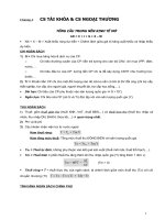
A Monetary Injection

Interest
rate

In panel (a), an increase in the money supply from MS1 to MS2 reduces the equilibrium interest
rate from r1 to r2. Because the interest rate is the cost of borrowing, the fall in the interest rate
raises the quantity of goods and services demanded at a given price level from Y1 to Y2. Thus,
in panel (b), the aggregate-demand curve shifts to the right from AD1 to AD2.

Quantity
of money
0

(a) The Money Market

Price
level

Quantity of output
0

(b) The Aggregate-Demand Curve

Aggregate
demand, AD1
Money demand

at price level P
Money supply,

MS1

r1

Y1
P

1. When the Fed
increases the
money supply . . .
MS2

r2

AD2

Y2
2. . . . the equilibrium

</div>
(22)<div class='page_container' data-page=22>

Liquidity Trap & Monetary Policy

• Liquidity Trap

?

• [

Lãi suất quá thấp

(

tiệm cận

zero) do

vậy chính sách tiền tệ thơng thường mất

tác dụng

]

• Deflation and Liquidity Trap

?

• [

Tại

sao

giảm phát và bẫy

thanh

khoản trở thành vòng xoắn đi xuống

?]

</div>
(23)<div class='page_container' data-page=23>

Giảm phát và bẫy

thanh

khoản

Giảm phát

(Deflation)

Bẫy

thanh

khoản

(Liquidity trap)

Giảm

phát

Bẫy

thanh

</div>
(24)<div class='page_container' data-page=24>

Hiệu ứng

Fisher

Phương trình

Fisher (

Fisher equation

)

i = r + %

Δ

P

(e)

• %

Δ

P = 6%

• i = 7%

=> r = 1%

Hiệu ứng

Fisher (

Fisher effect

)

• i = r + %

Δ

P

e

1:1

Khi NHTU t

ă

ng

tốc

độ

t

ă

ng tr

ưở

ng

tiền

,

kết quả

dài hạn

Tỷ lệ lạm phát

(%

Δ

P) cao h

ơ

n =>

</div>
(25)<div class='page_container' data-page=25>

Deflation



Liquidity Trap

• GFC 2008 => economic depression => AD? => P? = %

Δ

P? [

Deflation

]

• Fisher effect: i = r + %

Δ

P

[%

Δ

P => i]

#

[1:1]

• %

Δ

P? => i

? (but i: “zero bound”) =>

Liquidity Trap

!

•

0 = r + (-1);

0 = r + (-

2)…

=> r = ?

• r => C, I… => AD? => [

Deflation

]

• And so on

…

Solution

:

• QE (Quantitative Easing) + …[

not

OMO (Open Market Operations)]

• US vs. Japan & Euro

Giảm

phát

Bẫy

thanh

</div>
(26)<div class='page_container' data-page=26>

Using Policy for Stabilization

(?)

• Keynes

• Key role of AD in explaining short-run economic fluctuations

• The

government should actively stimulate aggregate demand

• When AD appeared insufficient to maintain production at its full-employment level

• Case

against active

stabilization policy

• Government

• Should avoid

active use of monetary and fiscal policy

• To try to stabilize the economy

• Affect the economy with a

big lag

(Time lags = Inside lags + outside lags)

</div>
(27)<div class='page_container' data-page=27>

Stabilization Policy

–

Time Lags

• Time lags = Inside lags + outside lags

Phát hiện trục trặc

Biện pháp

can

thiệp

Phát

huy

tác dụng

Độ trễ

trong

(Inside lags)

Độ trễ ngồi

(Outside lags)

Fiscal Policy

(

Chính sách tài khóa

)

*

Monetary Policy

</div>
(28)<div class='page_container' data-page=28>

Macroeconomic Policy

–

Stabilization the

Economy?

• Should Policy be:

Active

(?) or.

Passive

(?)

• Lags in the implementation and effects of policies (Time lags)

• The difficult jobs of economic forecasting

• Ignorance, expectations, and the Lucas critique

• If Active

: Should Policy be conducted by:

Rule

(?) or

Discretion

(?)

• Rule (?)

• Distrust

of policymakers and the political process.

• The time inconsistency of discretionary policy

.

• …

1. Japan: Deflation and %

Δ

P(Expectation)

2. Inflation Targeting (IT): 1990s, 2000s [%

Δ

P with buffer zone)

3. United States: Taylor’s Rule

</div>
(29)<div class='page_container' data-page=29></div>
(30)<div class='page_container' data-page=30>

Discussion

• Counter

-cyclical (monetary,

fiscal) policy

• Pro

-cyclical (monetary, fiscal)

policy

• Keynes

: Counter… or Pro…?

• Why:

Pro…?

How

: avoid?

A

</div>
(31)<div class='page_container' data-page=31>

Counter

-cyclical (monetary, fiscal) policy

Chính sách

nghịch

chu

kỳ

Kinh

tế đang hướng về

A

• Chính sách tài khóa

:

• G:

• T:

• Chính sách tiền tệ

:

• i:

• Ms:

Kinh

tế đang hướng về

B

• Chính sách tài khóa

:

• G:

• T:

• Chính sách tiền tệ

:

• i:

• Ms:

A

</div>
(32)<div class='page_container' data-page=32>

Bài giảng 4 (tiếp theo). Chính sách tài khóa và tiền tệ (Chỉ có bản tiếng Anh)

The Influence of Monetary Policy and

Fiscal Policy on AD

Châu Văn Thành

<b>Monetary Policy?</b>

<b>Fiscal Policy?</b>

Macroeconomics

•

<b>Economic growth </b>

–

longer trend

•

<b>Economic fluctuations </b>

–

short

run economic fluctuations

<b>Demand Management Policy</b>

<b># Stabilization Policy</b>

•

Monetary Policy

✓

Exchange Rate Policy

Tổng cầu

AD?

AD = C(Y-

<b>T</b>

) + I(

<b>r</b>

) +

<b>G</b>

+ X(

<b>ε</b>

,Y*) - M(

<b>ε</b>

,Y)

•

C = C(Y-

<b>T</b>

)

[

Hộ

gia

đình

]

•

<b>G</b>

[

Chính phủ

]

•

I = I(

<b>r</b>

)

[Doanh

nghiệp

] [ i = r + %

Δ

P],[

Ms

,

i

]

Fiscal Policy?

•

<b>Govt.</b>

(

T,G

) => AD => Y&

g

<sub>Y</sub>

, u, P&%

ΔP,…

•

T = NT = Net Taxes = Taxes

–

Govt. Transfers

•

Automatic Stabilizers

? (Taxes, Govt. Transfers)

•