Tài liệu Specification Error docx

Nguyeãn Troïng Hoaøi Analytical Methods 9
Specification Error
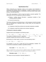
When constructing any regression model, we are always most interested in
explaining what variables cause the dependent variable to change and by how
much. This will always depend on a combination of economic theory; basic human
behavior; and past experience.
One of the assumptions of OLS is that the model is correctly specified. The
specification error can be explained by these two aspects : -
a) Missing / omitting relevant information / explanatory variables or from
including irrelevant variables.
b) Incorrect functional form.
This lecture will discuss the following issues : which regressors should be included
and / or excluded from a particular model. In other words, we will consider the
following cases : -
a) A regression model that excludes some important explanatory variables.
b) A regression model that includes some irrelevant regressors.
1) Exclusion of relevant variables
Suppose that we are interested in the following model : -
( ) ( ) ( ) ( )
1 2 2 K i
K 1 1 K L K L

i i Ki
K i i
Y X X X X
β β β β β ε
+ + + +
= + + + + + + +L L
The question is whether the set of L regressors -
( ) ( )
X X

L K 1 K ++
++ L
- are
important variables that should be included in the model.
But because of a certain reason, we have to use the following model : -
1 2 2 K i
+
i i Ki
Y X X
β β β ε
= + + +L
For illustration, we can use a model with only two explanatory variables. The
model with two explanatory variables is specified as follows : -
True model
ii33i221i
ε Xβ Xβ β Y +++=
9.1
Note: we assumed that X
2
and X
3
are the two important regressors that explain the dependent
variable Y, that is, we expect that
3
β
# 0. The model we use to estimate is as follows : -
Estimation model
ii221i
ε Xβ β Y ++=
9.2

This means we have excluded an important regressor X
3i
.
1
1
Nguyeãn Troïng Hoaøi Analytical Methods 9
The LS estimator of
2
β
ˆ
is.
∑
∑
=
2
i2
i2i
2
x
Yx
β
ˆ
9.3
Recall the lecture of Prof. Motahar in calculating the coefficient for regressor X
2
.
Important consequences of excluding important explanatory variables
a)
2 2
ˆ

E
β β
 
≠
 
and
2 2
ˆ
E
β β
 
=
 
if only if COV(X
2
,X
3
) = 0
To calculate the mathematical expectation of this estimate, we must substitute Y
i
with the formula for the true model, since our true model is 9.1 : -
[ ]
( )









+++=
=
∑
∑
2
i2
ii33i221i2i
2
x
ε Xβ Xβ β Y x
E β
ˆ
E
9.4
[ ]
∑
∑
+=
2
i2
i32i
322
x
Xx
β β β
ˆ
E
9.5
2i 3 2i 3

2 2
2 2
x x
i i
i i
X x
x x
=
∑ ∑
∑ ∑
9.6
We can easily prove 9.5 and its numerator COV(X
2
,X
3
)
b)
2
ˆ
β
is no longer explained as the direct effect (net) on the dependent variable Y.
Notice that when omitting relevant variables, the estimated coefficient of the
explanatory variable is insignificant in explaining the direct effect (net) on the
dependent variable. We prove this as follows : -
Recall the simple regression of Prof Motahar in defining the slope of

ii221i
ε Xβ β Y ++=
2i
2

2
2
x
i
i
Y
x
β
∧
=
∑
∑
9.7
So, if the simple regression is
3 1 22 2 i

i i
X X
β β ε
= + +
the coefficient of X
2
can
also be defined by the expression, in which,the estimator is : -
2i 3
22
2
2
x
i

i
X
x
β
∧
=
∑
∑
9.8
2
2
Nguyeãn Troïng Hoaøi Analytical Methods 9
This coefficient is the direct effect of X
2
on X
3


( )
2i 1 2 2 3 3 i
2
2
2
x

i i i
i
Y X X
x
β β β ε

β
∧
 
= + + +
=
 
 
 
∑
∑
n n n n n
1 2 3 2 2 2 2 3 2
i 1 i 1 i 1 i 1 i 1
2 1 2 3
n n n n n
2 2 2 2 2
2 2 2 2
1 1 1 1 1
ˆ

i i i i i i i i i i
i i i i i
i i i i i
x X x x X x X x
x x x x x
β β β ε ε
β β β β
= = = = =
= = = = =
 

+ + +
 
 
= = + + +
∑ ∑ ∑ ∑ ∑
∑ ∑ ∑ ∑ ∑
Now notice that
∑
=
n
1 i
i
x
=
)XX(
n
1 i
i
∑
=
−
= 0 vaø
∑∑
==
=
n
1 i
2
i
n

1 i
ii
xXx
as compared with : -
∑
∑
=
=
n
1 i
2
i
n
1 i
ii
x
Xx
=1
Thus,
n n n
2 2 2 3 2
i 1 i 1 i 1
2 2 3
n n n
2 2 2
2 2 2
1 1 1
ˆ

i i i i i i

i i i
i i i
x X x X x
x x x
ε
β β β
= = =
= = =
= + +
∑ ∑ ∑
∑ ∑ ∑
9.9
And we also have : -
n
2 2
i 1
/ ( , ) 0
i i
x n COV X
ε ε
=
= =
∑
According to infinite samples and OLS assumptions we
have : -
2 2 3 22
ˆ
.
β β β β
∧

= +
9.10
Important meanings :
Gross effect of X
2
on Y in the model,
2
ˆ

β
equals the direct effect of X
2
on Y (that
is,
2
β
∧
in the true model) plus the indirect effect of X
2
on Y (that is,
3 22
.
β β
∧
).
Thus, the estimated coefficient in the regression without X
3
(and assuming that this
variable is relevant), so then
2

ˆ

β
is insignificant in explaining a direct effect (net)
on Y.
We can graphically illustrate this and address some examples.
3
3
Nguyeãn Troïng Hoaøi Analytical Methods 9

This regression shows that HOUSING is explained quite well through GNP and
INT.RATE. If we temporarily assume that this is the true model, we then regress
HOUSING against GNP.
4
4
Nguyeãn Troïng Hoaøi Analytical Methods 9

We can conclude that this model excluded an important explanatory variable -
INT.RATE (Observe how the coefficient of determination; the coefficient of GNP;
and the standard error of the estimator of GNP change).
Conduct another regression : INT.RATE on GNP
5
5