Tài liệu Physics exercises_solution:Chapter 02 doc

2.1: a) During the later 4.75-s interval, the rocket moves a distance
m63m1000.1
3

, and so the magnitude of the average velocity is
.sm197
s754
m63m1000.1
3


.
b)
sm169
s5.90
m1000.1
3


2.2: a) The magnitude of the average velocity on the return flight is
.sm42.4
)das400,86()da5.13(
)m105150(
3


The direction has been defined to be the –x-direction
).
ˆ
( i
b) Because the bird ends up at the starting point, the average velocity for the round

trip is 0.
2.3: Although the distance could be found, the intermediate calculation can be avoided
by considering that the time will be inversely proportional to the speed, and the extra time
will be
min.701
hrkm70
hrkm105
min)140(










2.4: The eastward run takes
)sm5.0m200(
= 40.0 s and the westward run takes
)sm4.0m280(
= 70.0 s. a) (200 m + 280 m)/(40.0 s + 70.0 s) =
sm4.4
to two
significant figures. b) The net displacement is 80 m west, so the average velocity is
)s110.0m80(
=
sm73.0
in the –x-direction

).
ˆ
( i
2.5: In time t the fast runner has traveled 200 m farther than the slow runner:
s286so,s)m(6.20m200s)m50.5(  ttt
.
Fast runner has run
m.1770)sm20.6( t
Slow runner has run
m.1570)sm50.5( t
2.6: The s-waves travel slower, so they arrive 33 s after the p-waves.
km250
s33
5.65.3
s33
s33
s
km
s
km
ps
ps





d
dd
v

d
v
d
v
d
tvtd
tt
2.7: a) The van will travel 480 m for the first 60 s and 1200 m for the next 60 s, for a
total distance of 1680 m in 120 s and an average speed of
.sm0.14
b) The first stage of
the journey takes
s30
sm8.0
m240

and the second stage of the journey takes
,s12s)m20m240( 
so the time for the 480-m trip is 42 s, for an average speed of
.sm11.4
c) The first case (part (a)); the average speed will be the numerical average
only if the time intervals are the same.
2.8: From the expression for x(t), x(0) = 0, x(2.00 s) = 5.60 m and x(4.00 s) = 20.8 m. a)
sm80.2
s2.00
0m60.5


b)
sm2.5

s4.00
0m8.20


c)
sm6.7
s2.00
m5.60m8.20


2.9: a) At
0 ,0
11
 xt
, so Eq (2.2) gives
.sm0.12
s)0.10(
s)0.10)(sm120.0(s)0.10)(sm4.2(
3
3
22
2
2
av



t
x
v

b) From Eq. (2.3), the instantaneous velocity as a function of time is
,)sm360.0()sm80.4(32
2
3
22
ttctbtv
x

so i)
,0)0( 
x
v
ii)
,sm0.15s)0.5)(sm360.0()s0.5)(sm80.4()s0.5(
2
32

x
v
and iii)
.sm0.12s)0.10)(sm360.0()s0.10)(sm80.4()s0.10(
2
32

x
v
c) The car is at rest when
0
x
v

. Therefore
0)sm360.0()sm80.4(
2
32
 tt
. The
only time after
0t
when the car is at rest is
s3.13
3
2
sm360.0
sm80.4
t
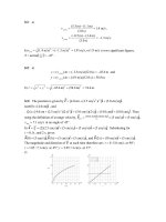
2.10: a) IV: The curve is horizontal; this corresponds to the time when she stops. b) I:
This is the time when the curve is most nearly straight and tilted upward (indicating
postive velocity). c) V: Here the curve is plainly straight, tilted downward (negative
velocity). d) II: The curve has a postive slope that is increasing. e) III: The curve is still
tilted upward (positive slope and positive velocity), but becoming less so.
2.11: Time (s) 0 2 4 6 8 10 12 14
16
Acceleration (m/s
2
) 0 1 2 2 3 1.5 1.5 0
a) The acceleration is not constant, but is approximately constant between the times
s4t
and
s.8t
2.12: The cruising speed of the car is 60

hrkm
= 16.7
sm
. a)
2
s10
sm7.16
sm7.1
(to
two significant figures). b)
2
s10
sm7.160
sm7.1

c) No change in speed, so the acceleration
is zero. d) The final speed is the same as the initial speed, so the average acceleration is
zero.
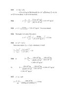
2.13: a) The plot of the velocity seems to be the most curved upward near t = 5 s.
b) The only negative acceleration (downward-sloping part of the plot) is between t = 30 s
and t = 40 s. c) At t = 20 s, the plot is level, and in Exercise 2.12 the car is said to be
cruising at constant speed, and so the acceleration is zero. d) The plot is very nearly a
straight line, and the acceleration is that found in part (b) of Exercise 2.12,
.sm7.1
2

e)
2.14: (a) The displacement vector is:
 
kjir

ˆ
)sm0.3()sm0.7(
ˆ
)sm0.10(
ˆ
)sm0.5()(
22
ttttt 

The velocity vector is the time derivative of the displacement vector:
kji
r
ˆ
))sm0.3(2sm0.7(
ˆ
)sm0.10(
ˆ
)sm0.5(
)(
2
t
dt
td


and the acceleration vector is the time derivative of the velocity vector:
k
r
ˆ
sm0.6

)(
2
2
2

dt
td

At t = 5.0 s:
 
kjir
ˆ
)s0.25)(sm0.3()s0.5)(sm0.7(
ˆ
)s0.5)(sm0.10(
ˆ
s)05)(sm0.5()(
2
2
 .t



kji
ˆ
)m0.40(
ˆ
)m0.50(
ˆ
)m0.25( 

kji
kji
r
ˆ
)sm0.23(
ˆ
)sm0.10(
ˆ
)sm0.5(
ˆ
))s0.5)(sm0.6(sm0.7((
ˆ
)sm0.10(
ˆ
)sm0.5(
)(
2


dt
td

k
r
ˆ
sm0.6
)(
2
2

2

dt
td

(b) The velocity in both the x- and the y-directions is constant and nonzero; thus
the overall velocity can never be zero.
(c) The object's acceleration is constant, since t does not appear in the acceleration
vector.
2.15:
t
dt
dx
v
x
)scm125.0(scm00.2
2

2
scm125.0
dt
dv
a
x
x
a)
.scm125.0,scm00.2cm,0.50,0At
2

xx

avxt
b)
s.0.16:for solveand0Set  ttv
x
c) Set x = 50.0 cm and solve for t. This gives
s.0.32 and0  tt
The turtle returns
to the starting point after 32.0 s.
d) Turtle is 10.0 cm from starting point when x = 60.0 cm or x = 40.0 cm.
s.8.25ands20.6:for solveandcm0.60Set  tttx
.scm23.1s,8.25At
.scm23.1s,20.6At


x
x
vt
vt
Set
cm0.40x
and solve for
s4.36: tt
(other root to the quadratic equation is negative
and hence nonphysical).
.scm55.2 s,4.36At 
x
vt
e)
2.16: Use of Eq. (2.5), with t = 10 s in all cases,
a)

      
2
m/s0.1s10/m/s0.15m/s0.5 
b)
      
2
m/s0.1s10/m/s0.5m/s0.15 
c)
      
2
m/s0.3s10/m/s0.15m/s0.15 
.
In all cases, the negative acceleration indicates an acceleration to the left.
2.17: a) Assuming the car comes to rest from 65 mph (29 m/s) in 4 seconds,
.sm25.7)s4()0sm29(
2

x
a
b) Since the car is coming to a stop, the acceleration is in the direction opposite to the
velocity. If the velocity is in the positive direction, the acceleration is negative; if the
velocity is in the negative direction, the acceleration is positive.
2.18: a) The velocity at t = 0 is
(3.00
sm
) + (0.100
3
sm
) (0) = 3.00
sm

,
and the velocity at t = 5.00 s is
(3.00
sm
) + (0.100
3
sm
) (5.00 s)
2
= 5.50
sm
,
so Eq. (2.4) gives the average acceleration as
2
sm50.
)s00.5(
)sm00.3()sm50.5(


.
b) The instantaneous acceleration is obtained by using Eq. (2.5),
.)sm2.0(2
3
tt
dt
dv
a
x



Then, i) at t = 0, a
x
= (0.2
3
sm
) (0) = 0, and
ii) at t = 5.00 s, a
x
= (0.2
3
sm
) (5.00 s) = 1.0
2
sm
.
2.19: a)
b)
2.20: a) The bumper’s velocity and acceleration are given as functions of time by
5
62
)sm600.0()sm60.9( tt
dt
dx
v
x

.)sm000.3()sm60.9(
4
62
t

dt
dv
a
x

There are two times at which v = 0 (three if negative times are considered), given by t =
0 and t
4
= 16 s
4
. At t = 0, x = 2.17 m and a
x
= 9.60
sm
2
. When t
4
= 16 s
4
,
x = (2.17 m) + (4.80
sm
2
)
)s16(
4
– (0.100)
6
sm
)(16 s

4
)
3/2
= 14.97 m,
a
x
= (9.60
sm
2
) – (3.000
6
sm
)(16 s
4
) = –38.4
sm
2
.
b)
2.21: a) Equating Equations (2.9) and (2.10) and solving for v
0
,
.sm00.5sm0.15
s007
m)70(2
)(2
0
0




.
v
t
xx
v
xx
b) The above result for v
0x
may be used to find
,sm43.1
s00.7
sm00.5sm0.15
2
0





t
vv
a
xx
x
or the intermediate calculation can be avoided by combining Eqs. (2.8) and (2.12) to
eliminate v
0x
and solving for a
x

,
.sm43.1
s)007(
m0.70
s00.7
sm0.15
22
2
22
0


















.t
xx

t
v
a
x
x
2.22: a) The acceleration is found from Eq. (2.13), which
x
v
0
= 0;
  
  
,sm0.32
)ft307(2
)hrmi173(
)(2
2
ft3.281
m1
2
hrmi1
sm4470.0
0
2



xx
v
a

x
x
where the conversions are from Appendix E.
b) The time can be found from the above acceleration,
 
.s42.2
sm0.32
)hrmi173(
2
hrmi1
sm4470.0

x
x
a
v
t
The intermediate calculation may be avoided by using Eq. (2.14), again with v
0x
= 0,
  
 
.s42.2
)hrmi173(
ft307(2
)(2
hrmi1
sm4470.0
ft3.281
m1

0



x
v
xx
t
2.23: From Eq. (2.13), with
 
,0 Taking.,0
0max
2
0
2
0


xaav
xx
v
xx
m.70.1
)sm250(2
))hrkms)(3.6mhr)(1km105((
2
2
2
max
2

0

a
v
x
x
2.24: In Eq. (2.14), with x – x
0
being the length of the runway, and v
0x
= 0 (the plane
starts from rest),
.sm0.7022
s8
m280
0


t
xx
x
v
2.25: a) From Eq. (2.13), with
,0
0

x
v
.sm67.1
m)120(2

)sm20(
)(2
2
2
0
2



xx
v
a
x
x
b) Using Eq. (2.14),
s.12)sm20(m)120(2)(2
0
 vxxt
c)
m.240)sm20)(s12( 
2.26: a) x
0
< 0, v
0x
< 0, a
x
< 0
b) x
0
> 0, v

0x
< 0, a
x
> 0
c) x
0
> 0, v
0x
> 0, a
x
< 0
2.27: a) speeding up:
?s,9.19,0ft,1320
00

xx
atvxx
22
2
1
00
sft67.6gives 
xxx
atatvxx
slowing down:
?,0,sft0.88ft,146
00

xxx
avvxx

.sft5.26gives)(2
2
0
2
0
2

xxxx
axxavv
b)
? ,sft676,0ft,1320
2
00

xxx
v.avxx
.mph5.90sft133gives)(2
0
2
0
2

xxxx
vxxavv
constant.benot must
x
a
c)
?,0,sft5.26 s,ft0.88
2

0
 tvav
xxx
s.32.3gives
0
 ttavv
xxx
2.28: a) Interpolating from the graph:
left) the(toscm3.1,s0.7At
right) the(toscm72s,0.4At


v
.v
b)
2
s0.6
s/cm0.8
scm3.1graph-ofslope  tva
which is constant
c)
x
area under v-t graph
First 4.5 s:
TriangleRectangle
AAx 
   
cm5.22
s
cm

6s5.4
2
1
s
cm
2s5.4















From 0 to 7.5 s:
The distance is the sum of the magnitudes of the areas.
   
cm5.25
s
cm
2s5.1
2
1

s
cm
8s6
2
1















d
d)
2.29: a)
b)
2.30: a)
2.31: a) At t = 3 s the graph is horizontal and the acceleration is 0. From t = 5 s to t =
9 s, the acceleration is constant (from the graph) and equal to
2
s4
sm20sm45

sm3.6

. From
t = 9 s to t = 13 s the acceleration is constant and equal to
.sm2.11
2
s4
sm450


b) In the first five seconds, the area under the graph is the area of the rectangle, (20
m)(5 s) = 100 m. Between t = 5 s and t = 9 s, the area under the trapezoid is (1/2)(45 m/s
+ 20 m/s)(4 s) = 130 m (compare to Eq. (2.14)), and so the total distance in the first 9 s is
230 m. Between t = 9 s and t = 13 s, the area under the triangle is
m90s)4)(sm45)(21( 
, and so the total distance in the first 13 s is 320 m.
2.32:
2.33: a) The maximum speed will be that after the first 10 min (or 600 s), at which time
the speed will be
.skm18sm101.8s)900)(sm0.20(
4
2

b) During the first 15 minutes (and also during the last 15 minutes), the ship will travel
km8100s)900)(skm18)(21( 
, so the distance traveled at non-constant speed is 16,200
km and the fraction of the distance traveled at constant speed is
,958.0
km384,000
km200,16

1

keeping an extra significant figure.
c) The time spent at constant speed is
s1004.2
4
skm18
km200,16km000,384


and the time spent
during both the period of acceleration and deceleration is 900 s, so the total time required
for the trip is
s102.22
4

, about 6.2 hr.
2.34: After the initial acceleration, the train has traveled
m8.156)s0.14)(sm60.1(
2
1
2
2

(from Eq. (2.12), with x
0
= 0, v
0x
= 0), and has attained a speed of
.sm4.22)s0.14)(sm60.1(

2

During the 70-second period when the train moves with constant speed, the train travels
  
m.1568s70sm4.22 
The distance traveled during deceleration is given by Eq.
(2.13), with
sm4.22,0
0

xx
vv
and
2
sm50.3
x
a
, so the train moves a distance
.m68.71
)m/s3.502(
)s/m4.22(
0
2
2



xx
The total distance covered in then 156.8 m + 1568 m + 71.7 m
= 1.8 km.

In terms of the initial acceleration a
1
, the initial acceleration time t
1
, the time t
2
during
which the train moves at constant speed and the magnitude a
2
of the final acceleration,
the total distance x
T
is given by
which yields the same result.
,
||
2
2||
)(
2
1
)(
2
1
2
11
21
11
2
2

11
211
2
11T
















a
ta
tt
ta
a
ta
ttatax
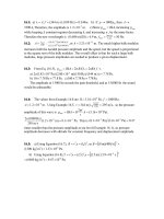
2.35: a)
b) From the graph (Fig. (2.35)), the curves for A and B intersect at t = 1 s and t = 3 s.
c)

d) From Fig. (2.35), the graphs have the same slope at t = 2 s . e) Car A passes car B
when they have the same position and the slope of curve A is greater than that of curve B
in Fig. (2.30); this is at t = 3 s. f) Car B passes car A when they have the same position
and the slope of curve B is greater than that of curve A; this is at t = 1 s.
2.36: a) The truck’s position as a function of time is given by x
T
= v
T
t, with v
T
being the
truck’s constant speed, and the car’s position is given by x
C
= (1/2) a
C
t
2
. Equating the
two expressions and dividing by a factor of t (this reflects the fact that the car and the
truck are at the same place at t = 0) and solving for t yields
s5.12
sm20.3
)sm0.20(2
2
2
C
T

a
v

t
and at this time
x
T
= x
C
= 250 m.
b) a
C
t = (3.20 m/s
2
)(12.5 s) = 40.0 m/s (See Exercise 2.37 for a discussion of why the
car’s speed at this time is twice the truck’s speed.)
c)
d)
2.37: a)
The car and the motorcycle have gone the same distance during the same time, so their
average speeds are the same. The car's average speed is its constant speed v
C
, and for
constant acceleration from rest, the motorcycle's speed is always twice its
average, or 2v
C
. b) From the above, the motorcyle's speed will be v
C
after half the time
needed to catch the car. For motion from rest with constant acceleration, the distance
traveled is proportional to the square of the time, so for half the time
one-fourth of the total distance has been covered, or
.4d

2.38: a) An initial height of 200 m gives a speed of 60
sm
when rounded to one
significant figure. This is approximately 200 km/hr or approximately 150
hrmi
.
(Different values of the approximate height will give different answers; the above may be
interpreted as slightly better than order of magnitude answers.) b) Personal experience
will vary, but speeds on the order of one or two meters per second are reasonable. c) Air
resistance may certainly not be neglected.
2.39: a) From Eq. (2.13), with
0
y
v
and
ga
y

,
,sm94.2m)440.0)(sm80.9(2)(2
2
00
 yygv
y
which is probably too precise for the speed of a flea; rounding down, the speed is about
sm9.2
.
b) The time the flea is rising is the above speed divided by g, and the total time is twice
this; symbolically,
s,599.0

)m/s(9.80
)m440.0(2
2
)(2
2
)(2
2
2
0
0





g
yy
g
yyg
t
or about 0.60 s.
2.40: Using Eq. (2.13), with downward velocities and accelerations being positive,
2
y
v
=
(0.8
sm
)
2

+ 2(1.6
2
sm
)(5.0 m) = 16.64
22
sm
(keeping extra significant figures), so v
y
= 4.1
sm
.
2.41: a) If the meter stick is in free fall, the distance d is related to the reaction time t by
2
)21( gtd 
, so
.2 gdt 
If d is measured in centimeters, the reaction time is
.cm)1(s)1052.4(
scm980
22
2
2
ddd
g
t


b) Using the above result,
s.190.017.6s)1052.4(
2



2.42: a)
m.6.30s)5.2)(sm80.9)(21()21(
222
gt
b)
sm.5.24s)5.2)(sm80.9(
2
gt
.
c)
2.43: a) Using the method of Example 2.8, the time the ring is in the air is
)sm80.9(
)m0.12()sm80.9(2s)m00.5(s)m00.5(
)(2
2
2
2
0
2
00




g
yygvv
t
yy

s,156.2
keeping an extra significant figure. The average velocity is then
sm57.5
s2.156
m0.12

, down.
As an alternative to using the quadratic formula, the speed of the ring when it hits the
ground may be obtained from
)(2
0
2
0
2
yygvv
yy

, and the average velocity found
from
2
0 yy
vv 
; this is algebraically identical to the result obtained by the quadratic formula.
b) While the ring is in free fall, the average acceleration is the constant acceleration due
to gravity,
2
s/m80.9
down.
c)

2
00
2
1
gttvyy
y

22
)sm8.9(
2
1
)sm(5.00m0.120
tt 
Solve this quadratic as in part a) to obtain t = 2.156 s.
d)
)m0.12)(sm8.9(2)sm(5.00)(2
22
0
2
0
2
 yygvv
yy

sm1.16
y
v
e)
2.44: a) Using a
y

= –g, v
0y
= 5.00
sm
and y
0
= 40.0 m in Eqs. (2.8) and (2.12) gives
i) at t = 0.250 s,
y = (40.0 m) + (5.00
sm
)(0.250 s) – (1/2)(9.80
2
sm
)(0.250 s)
2
= 40.9 m,
v
y
= (5.00
sm
) – (9.80
2
sm
)(0.250 s) = 2.55
sm
and ii) at t = 1.00 s,
y = (40.0 m) + (5.00 m/s)(1.00 s) – (1/2)(9.80 m/s
2
)(1.00 s)
2

= 40.1 m,
v
y
= (5.00
sm
) – (9.80
2
sm
)(1.00 s) = – 4.80
sm
.
b) Using the result derived in Example 2.8, the time is
t =
)sm80.9(
)m0.400)(sm80.9(2)sm00.5()sm00.5(
2
2
2

= 3.41 s.
c) Either using the above time in Eq. (2.8) or avoiding the intermediate calculation by
using Eq. (2.13),
,sm809)m0.40)(sm80.9(2)sm00.5()(2
2
2
2
2
0
2
0

2
 yygvv
yy
v
y
= 28.4
sm
.
d) Using v
y
= 0 in Eq. (2.13) gives
.m2.41m0.40
)sm80.9(2
)sm00.5(
2
2
2
0
2
0
 y
g
v
y
e)
2.45: a)
,sm6.25s)00.2)(sm80.9()sm00.6(
2
0
 gtvv

yy
so the speed is
sm6.25
.
b)
m,6.31s)00.2)(sm80.9(
2
1
s)00.2)(sm00.6(
2
1
2
2
2
0
 gttvy
y
with the
minus sign indicating that the balloon has indeed fallen.
c)
m2.15so,sm232m)0.10)(sm80.9(2s)m00.6()(2
2222
0
2
0
2

yyy
vyygvv
2.46: a) The vertical distance from the initial position is given by

;
2
1
2
0
gttvy
y

solving for v
0y
,
.sm5.14)s00.5)(sm80.9(
2
1
)s00.5(
)m0.50(
2
1
2
0


 gt
t
y
v
y
b) The above result could be used in
 
,2

0
2
0
2
yygvv
yy

with v = 0, to solve for y
– y
0
= 10.7 m (this requires retention of two extra significant figures in the calculation
for v
0y
). c) 0 d) 9.8
2
sm
, down.
e) Assume the top of the building is 50 m above the ground for purposes of graphing:
2.47: a)
.sm249s)9.0()sm224(
2

b)
.4.25
2
2
sm9.80
sm249

c) The most direct way to

find the distance is
m.101s)9.0)(2)sm224((
ave
tv

d)
22
sm39240butsm202)s40.1()sm283(  g
, so the figures are not consistent.
2.48: a) From Eq. (2.8), solving for t gives (40.0
sm
– 20.0
sm
)/9.80
2
sm
= 2.04 s.
b) Again from Eq. (2.8),
.s12.6
sm80.9
)sm0.20(sm0.40
2



c) The displacement will be zero when the ball has returned to its original vertical
position, with velocity opposite to the original velocity. From Eq. (2.8),
.s16.8
sm80.9
)sm40(sm40

2


(This ignores the t = 0 solution.)
d) Again from Eq. (2.8), (40
sm
)/(9.80
2
sm
) = 4.08 s. This is, of course, half the
time found in part (c).
e) 9.80
2
sm
, down, in all cases.
f)
2.49: a) For a given initial upward speed, the height would be inversely proportional to
the magnitude of g, and with g one-tenth as large, the height would be ten times higher,
or 7.5 m. b) Similarly, if the ball is thrown with the same upward speed, it would go ten
times as high, or 180 m. c) The maximum height is determined by the speed when hitting
the ground; if this speed is to be the same, the maximum height would be ten times as
large, or 20 m.
2.50: a) From Eq. (2.15), the velocity v
2
at time t



t
t

dtαtvv
1
12
)(
2
2
1
2
1
ttv 

22
11
22
ttv


= (5.0
sm
) – (0.6
3
sm
)(1.0 s)
2
+ (0.6
3
sm
) t
2
= (4.40

sm
) + (0.6
3
sm
) t
2
.
At t
2
= 2.0 s, the velocity is v
2
= (4.40
sm
) + (0.6
3
sm
)(2.0 s)
2
= 6.80 m/s, or 6.8
sm
to two significant figures.
b) From Eq. (2.16), the position x
2
as a function of time is

dtvxx
x
t
t
1

12

dtt
t
t
))s/m6.0()s/m40.4(()m0.6(
23
1

).(
3
)sm6.0(
))(sm40.4()m0.6(
3
1
3
3
1
tttt 
At t = 2.0 s, and with t
1
= 1.0 s,
x = (6.0 m) + (4.40
sm
)((2.0 s) – (1.0 s)) + (0.20
3
sm
)((2.0 s)
3
– (1.0 s)

3
)
= 11.8 m.
c)