Tài liệu Adaptive Live Signal and Image Processing pdf
Bạn đang xem bản rút gọn của tài liệu. Xem và tải ngay bản đầy đủ của tài liệu tại đây (24.17 MB, 587 trang )
Adaptive
Blind Signal
and
Image Processing
Learning Algorithms
and Applications
includes CD
Andrzej CICHOCKI Shun-ichi AMARI
Contents
Preface xxix
1 Introduction to Blind Signal Processing: Problems and Applications 1
1.1 Problem Formulations – An Overview 2
1.1.1 Generalized Blind Signal Processing Problem 2
1.1.2 Instantaneous Blind Source Separation and
Independent Component Analysis 5
1.1.3 Independent Component Analysis for Noisy Data 11
1.1.4 Multichannel Blind Deconvolution and Separation 14
1.1.5 Blind Extraction of Signals 18
1.1.6 Generalized Multichannel Blind Deconvolution –
State Space Models 19
1.1.7 Nonlinear State Space Models – Semi-Blind Signal
Processing 21
1.1.8 Why State Space Demixing Models? 22
1.2 Potential Applications of Blind and Semi-Blind Signal
Processing 23
1.2.1 Biomedical Signal Processing 24
1.2.2 Blind Separation of Electrocardiographic Signals of
Fetus and Mother 25
1.2.3 Enhancement and Decomposition of EMG Signals 27
v
vi CONTENTS
1.2.4 EEG and Data MEG Processing 27
1.2.5 Application of ICA/BSS for Noise and Interference
Cancellation in Multi-sensory Biomedical Signals 29
1.2.6 Cocktail Party Problem 34
1.2.7 Digital Communication Systems 35
1.2.7.1 Why Blind? 37
1.2.8 Image Restoration and Understanding 37
2 Solving a System of Algebraic Equations and Related Problems 43
2.1 Formulation of the Problem for Systems of Linear Equations 44
2.2 Least-Squares Problems 45
2.2.1 Basic Features of the Least-Squares Solution 45
2.2.2 Weighted Least-Squares and Best Linear Unbiased
Estimation 47
2.2.3 Basic Network Structure-Least-Squares Criteria 49
2.2.4 Iterative Parallel Algorithms for Large and Sparse
Systems 49
2.2.5 Iterative Algorithms with Non-negativity Constraints 51
2.2.6 Robust Circuit Structure by Using the Interactively
Reweighted Least-Squares Criteria 54
2.2.7 Tikhonov Regularization and SVD 57
2.3 Least Absolute Deviation (1-norm) Solution of Systems of
Linear Equations 61
2.3.1 Neural Network Architectures Using a Smooth
Approximation and Regularization 62
2.3.2 Neural Network Model for LAD Problem Exploiting
Inhibition Principles 64
2.4 Total Least-Squares and Data Least-Squares Problems 67
2.4.1 Problems Formulation 67
2.4.1.1 A Historical Overview of the TLS Problem 67
2.4.2 Total Least-Squares Estimation 69
2.4.3 Adaptive Generalized Total Least-Squares 73
2.4.4 Extended TLS for Correlated Noise Statistics 75
2.4.4.1 Choice of
¯
R
NN
in Some Practical Situations 77
2.4.5 Adaptive Extended Total Least-Squares 77
2.4.6 An Illustrative Example - Fitting a Straight Line to a
Set of Points 78
2.5 Sparse Signal Representation and Minimum Fuel Consumption
Problem 79
CONTENTS vii
2.5.1 Approximate Solution of Minimum Fuel Problem
Using Iterative LS Approach 81
2.5.2 FOCUSS Algorithms 83
3 Principal/Minor Component Analysis and Related Problems 87
3.1 Introduction 87
3.2 Basic Properties of PCA 88
3.2.1 Eigenvalue Decomposition 88
3.2.2 Estimation of Sample Covariance Matrices 90
3.2.3 Signal and Noise Subspaces - AIC and MDL Criteria
for their Estimation 91
3.2.4 Basic Properties of PCA 93
3.3 Extraction of Principal Components 94
3.4 Basic Cost Functions and Adaptive Algorithms for PCA 98
3.4.1 The Rayleigh Quotient – Basic Properties 98
3.4.2 Basic Cost Functions for Computing Principal and
Minor Components 99
3.4.3 Fast PCA Algorithm Based on the Power Method 101
3.4.4 Inverse Power Iteration Method 104
3.5 Robust PCA 104
3.6 Adaptive Learning Algorithms for MCA 107
3.7 Unified Parallel Algorithms for PCA/MCA and PSA/MSA 110
3.7.1 Cost Function for Parallel Processing 111
3.7.2 Gradient of J(W) 112
3.7.3 Stability Analysis 113
3.7.4 Unified Stable Algorithms 116
3.8 SVD in Relation to PCA and Matrix Subspaces 118
3.9 Multistage PCA for BSS 119
Appendix A. Basic Neural Networks Algorithms for Real and
Complex-Valued PCA 122
Appendix B. Hierarchical Neural Network for Complex-valued
PCA 125
4 Blind Decorrelation and SOS for Robust Blind Identification 129
4.1 Spatial Decorrelation - Whitening Transforms 130
4.1.1 Batch Approach 130
4.1.2 Optimization Criteria for Adaptive Blind Spatial
Decorrelation 132
viii CONTENTS
4.1.3 Derivation of Equivariant Adaptive Algorithms for
Blind Spatial Decorrelation 133
4.1.4 Simple Local Learning Rule 136
4.1.5 Gram-Schmidt Orthogonalization 138
4.1.6 Blind Separation of Decorrelated Sources Versus
Spatial Decorrelation 139
4.1.7 Bias Removal for Noisy Data 139
4.1.8 Robust Prewhitening - Batch Algorithm 140
4.2 SOS Blind Identification Based on EVD 141
4.2.1 Mixing Model 141
4.2.2 Basic Principles: SD and EVD 143
4.3 Improved Blind Identification Algorithms Based on
EVD/SVD 148
4.3.1 Robust Orthogonalization of Mixing Matrices for
Colored Sources 148
4.3.2 Improved Algorithm Based on GEVD 153
4.3.3 Improved Two-stage Symmetric EVD/SVD Algorithm 155
4.3.4 BSS and Identification Using Bandpass Filters 156
4.4 Joint Diagonalization - Robust SOBI Algorithms 157
4.4.1 Modified SOBI Algorithm for Nonstationary Sources:
SONS Algorithm 160
4.4.2 Computer Simulation Experiments 161
4.4.3 Extensions of Joint Approximate Diagonalization
Technique 162
4.4.4 Comparison of the JAD and Symmetric EVD 163
4.5 Cancellation of Correlation 164
4.5.1 Standard Estimation of Mixing Matrix and Noise
Covariance Matrix 164
4.5.2 Blind Identification of Mixing Matrix Using the
Concept of Cancellation of Correlation 165
Appendix A. Stability of the Amari’s Natural Gradient and
the Atick-Redlich Formula 168
Appendix B. Gradient Descent Learning Algorithms with
Invariant Frobenius Norm of the Separating Matrix 171
Appendix C. JADE Algorithm 173
5 Sequential Blind Signal Extraction 177
5.1 Introduction and Problem Formulation 178
5.2 Learning Algorithms Based on Kurtosis as Cost Function 180
CONTENTS ix
5.2.1 A Cascade Neural Network for Blind Extraction of
Non-Gaussian Sources with Learning Rule Based on
Normalized Kurtosis 181
5.2.2 Algorithms Based on Optimization of Generalized
Kurtosis 184
5.2.3 KuicNet Learning Algorithm 186
5.2.4 Fixed-point Algorithms 187
5.2.5 Sequential Extraction and Deflation Procedure 191
5.3 On Line Algorithms for Blind Signal Extraction of
Temporally Correlated Sources 193
5.3.1 On Line Algorithms for Blind Extraction Using
Linear Predictor 195
5.3.2 Neural Network for Multi-unit Blind Extraction 197
5.4 Batch Algorithms for Blind Extraction of Temporally
Correlated Sources 199
5.4.1 Blind Extraction Using a First Order Linear Predictor 201
5.4.2 Blind Extraction of Sources Using Bank of Adaptive
Bandpass Filters 202
5.4.3 Blind Extraction of Desired Sources Correlated with
Reference Signals 205
5.5 Statistical Approach to Sequential Extraction of Independent
Sources 206
5.5.1 Log Likelihood and Cost Function 206
5.5.2 Learning Dynamics 208
5.5.3 Equilibrium of Dynamics 209
5.5.4 Stability of Learning Dynamics and Newton’s Method 210
5.6 Statistical Approach to Temporally Correlated Sources 212
5.7 On-line Sequential Extraction of Convolved and Mixed
Sources 214
5.7.1 Formulation of the Problem 214
5.7.2 Extraction of Single i.i.d. Source Signal 215
5.7.3 Extraction of Multiple i.i.d. Sources 217
5.7.4 Extraction of Colored Sources from Convolutive
Mixture 218
5.8 Computer Simulations: Illustrative Examples 219
5.8.1 Extraction of Colored Gaussian Signals 219
5.8.2 Extraction of Natural Speech Signals from Colored
Gaussian Signals 221
5.8.3 Extraction of Colored and White Sources 222
5.8.4 Extraction of Natural Image Signal from Interferences 223
x CONTENTS
5.9 Concluding Remarks 224
Appendix A. Global Convergence of Algorithms for Blind
Source Extraction Based on Kurtosis 225
Appendix B. Analysis of Extraction and Deflation Procedure 227
Appendix C. Conditions for Extraction of Sources Using
Linear Predictor Approach 228
6 Natural Gradient Approach to Independent Component Analysis 231
6.1 Basic Natural Gradient Algorithms 232
6.1.1 Kullback–Leibler Divergence - Relative Entropy as
Measure of Stochastic Independence 232
6.1.2 Derivation of Natural Gradient Basic Learning Rules 235
6.2 Generalizations of Basic Natural Gradient Algorithm 237
6.2.1 Nonholonomic Learning Rules 237
6.2.2 Natural Riemannian Gradient in Orthogonality
Constraint 239
6.2.2.1 Local Stability Analysis 240
6.3 NG Algorithms for Blind Extraction 242
6.3.1 Stiefel Manifolds Approach 242
6.4 Generalized Gaussian Distribution Model 243
6.4.1 The Moments of the Generalized Gaussian
Distribution 248
6.4.2 Kurtosis and Gaussian Exponent 249
6.4.3 The Flexible ICA Algorithm 250
6.4.4 Pearson Model 253
6.5 Natural Gradient Algorithms for Non-stationary Sources 254
6.5.1 Model Assumptions 254
6.5.2 Second Order Statistics Cost Function 255
6.5.3 Derivation of NG Learning Algorithms 255
Appendix A. Derivation of Local Stability Conditions for NG
ICA Algorithm (6.19) 258
Appendix B. Derivation of the Learning Rule (6.32) and
Stability Conditions for ICA 260
Appendix C. Stability of Generalized Adaptive Learning
Algorithm 262
Appendix D. Dynamic Properties and Stability of
Nonholonomic NG Algorithms 264
Appendix E. Summary of Stability Conditions 267
Appendix F. Natural Gradient for Non-square Separating
Matrix 268
CONTENTS xi
Appendix G. Lie Groups and Natural Gradient for General
Case 269
G.0.1 Lie Group Gl(n, m) 270
G.0.2 Derivation of Natural Learning Algorithm for m > n 271
7 Locally Adaptive Algorithms for ICA and their Implementations 273
7.1 Modified Jutten-H´erault Algorithms for Blind Separation of
Sources 274
7.1.1 Recurrent Neural Network 274
7.1.2 Statistical Independence 274
7.1.3 Self-normalization 277
7.1.4 Feed-forward Neural Network and Associated
Learning Algorithms 278
7.1.5 Multilayer Neural Networks 282
7.2 Iterative Matrix Inversion Approach to Derivation of Family
of Robust ICA Algorithms 285
7.2.1 Derivation of Robust ICA Algorithm Using
Generalized Natural Gradient Approach 288
7.2.2 Practical Implementation of the Algorithms 289
7.2.3 Special Forms of the Flexible Robust Algorithm 291
7.2.4 Decorrelation Algorithm 291
7.2.5 Natural Gradient Algorithms 291
7.2.6 Generalized EASI Algorithm 291
7.2.7 Non-linear PCA Algorithm 292
7.2.8 Flexible ICA Algorithm for Unknown Number of
Sources and their Statistics 293
7.3 Computer Simulations 294
Appendix A. Stability Conditions for the Robust ICA
Algorithm (7.50) [332] 300
8 Robust Techniques for BSS and ICA with Noisy Data 305
8.1 Introduction 305
8.2 Bias Removal Techniques for Prewhitening and ICA
Algorithms 306
8.2.1 Bias Removal for Whitening Algorithms 306
8.2.2 Bias Removal for Adaptive ICA Algorithms 307
8.3 Blind Separation of Signals Buried in Additive Convolutive
Reference Noise 310
8.3.1 Learning Algorithms for Noise Cancellation 311
8.4 Cumulants Based Adaptive ICA Algorithms 314
xii CONTENTS
8.4.1 Cumulants Based Cost Functions 314
8.4.2 Family of Equivariant Algorithms Employing the
Higher Order Cumulants 315
8.4.3 Possible Extensions 317
8.4.4 Cumulants for Complex Valued Signals 318
8.4.5 Blind Separation with More Sensors than Sources 318
8.5 Robust Extraction of Arbitrary Group of Source Signals 320
8.5.1 Blind Extraction of Sparse Sources with Largest
Positive Kurtosis Using Prewhitening and Semi-
Orthogonality Constraint 320
8.5.2 Blind Extraction of an Arbitrary Group of Sources
without Prewhitening 323
8.6 Recurrent Neural Network Approach for Noise Cancellation 325
8.6.1 Basic Concept and Algorithm Derivation 325
8.6.2 Simultaneous Estimation of a Mixing Matrix and
Noise Reduction 328
8.6.2.1 Regularization 329
8.6.3 Robust Prewhitening and Principal Component
Analysis (PCA) 331
8.6.4 Computer Simulation Experiments for Amari-
Hopfield Network 331
Appendix A. Cumulants in Terms of Moments 333
9 Multichannel Blind Deconvolution: Natural Gradient Approach 335
9.1 SIMO Convolutive Models and Learning Algorithms for
Estimation of Source Signal 336
9.1.1 Equalization Criteria for SIMO Systems 338
9.1.2 SIMO Blind Identification and Equalization via
Robust ICA/BSS 340
9.1.3 Feed-forward Deconvolution Model and Natural
Gradient Learning Algorithm 342
9.1.4 Recurrent Neural Network Model and Hebbian
Learning Algorithm 343
9.2 Multichannel Blind Deconvolution with Constraints Imposed
on FIR Filters 346
9.3 General Models for Multiple-Input Multiple-Output Blind
Deconvolution 349
9.3.1 Fundamental Models and Assumptions 349
9.3.2 Separation-Deconvolution Criteria 351
9.4 Relationships Between BSS/ICA and MBD 354
CONTENTS xiii
9.4.1 Multichannel Blind Deconvolution in the Frequency
Domain 354
9.4.2 Algebraic Equivalence of Various Approaches 355
9.4.3 Convolution as Multiplicative Operator 357
9.4.4 Natural Gradient Learning Rules for Multichannel
Blind Deconvolution (MBD) 358
9.4.5 NG Algorithms for Double Infinite Filters 359
9.4.6 Implementation of Algorithms for Minimum Phase
Non-causal System 360
9.4.6.1 Batch Update Rules 360
9.4.6.2 On-line Update Rule 360
9.4.6.3 Block On-line Update Rule 360
9.5 Natural Gradient Algorithms with Nonholonomic Constraints 362
9.5.1 Equivariant Learning Algorithm for Causal FIR
Filters in the Lie Group Sense 363
9.5.2 Natural Gradient Algorithm for Fully Recurrent
Network 367
9.6 MBD of Non-minimum Phase System Using Filter
Decomposition Approach 368
9.6.1 Information Back-propagation 370
9.6.2 Batch Natural Gradient Learning Algorithm 371
9.7 Computer Simulations Experiments 373
9.7.1 The Natural Gradient Algorithm vs. the Ordinary
Gradient Algorithm 373
9.7.2 Information Back-propagation Example 375
Appendix A. Lie Group and Riemannian Metric on FIR
Manifold 376
A.0.1 Lie Group 377
A.0.2 Riemannian Metric and Natural Gradient in the Lie
Group Sense 379
Appendix B. Properties and Stability Conditions for the
Equivariant Algorithm 381
B.0.1 Proof of Fundamental Properties and Stability
Analysis of Equivariant NG Algorithm (9.126) 381
B.0.2 Stability Analysis of the Learning Algorithm 381
10 Estimating Functions and Superefficiency for
ICA and Deconvolution 383
10.1 Estimating Functions for Standard ICA 384
10.1.1 What is Estimating Function? 384
xiv CONTENTS
10.1.2 Semiparametric Statistical Model 385
10.1.3 Admissible Class of Estimating Functions 386
10.1.4 Stability of Estimating Functions 389
10.1.5 Standardized Estimating Function and Adaptive
Newton Method 392
10.1.6 Analysis of Estimation Error and Superefficiency 393
10.1.7 Adaptive Choice of ϕ Function 395
10.2 Estimating Functions in Noisy Case 396
10.3 Estimating Functions for Temporally Correlated Source
Signals 397
10.3.1 Source Model 397
10.3.2 Likelihood and Score Functions 399
10.3.3 Estimating Functions 400
10.3.4 Simultaneous and Joint Diagonalization of Covariance
Matrices and Estimating Functions 401
10.3.5 Standardized Estimating Function and Newton
Method 404
10.3.6 Asymptotic Errors 407
10.4 Semiparametric Models for Multichannel Blind Deconvolution
407
10.4.1 Notation and Problem Statement 408
10.4.2 Geometrical Structures on FIR Manifold 409
10.4.3 Lie Group 410
10.4.4 Natural Gradient Approach for Multichannel Blind
Deconvolution 410
10.4.5 Efficient Score Matrix Function and its Representation
413
10.5 Estimating Functions for MBD 415
10.5.1 Superefficiency of Batch Estimator 418
Appendix A. Representation of Operator K(z) 419
11 Blind Filtering and Separation Using a State-Space Approach 423
11.1 Problem Formulation and Basic Models 424
11.1.1 Invertibility by State Space Model 427
11.1.2 Controller Canonical Form 428
11.2 Derivation of Basic Learning Algorithms 428
11.2.1 Gradient Descent Algorithms for Estimation of
Output Matrices W = [C, D] 429
11.2.2 Special Case - Multichannel Blind Deconvolution with
Causal FIR Filters 432
CONTENTS xv
11.2.3 Derivation of the Natural Gradient Algorithm for
State Space Model 432
11.3 Estimation of Matrices [A, B] by Information Back–
propagation 434
11.4 State Estimator – The Kalman Filter 437
11.4.1 Kalman Filter 437
11.5 Two–stage Separation Algorithm 439
Appendix A. Derivation of the Cost Function 440
12 Nonlinear State Space Models – Semi-Blind Signal Processing 443
12.1 General Formulation of The Problem 443
12.1.1 Invertibility by State Space Model 447
12.1.2 Internal Representation 447
12.2 Supervised-Unsupervised Learning Approach 448
12.2.1 Nonlinear Autoregressive Moving Average Model 448
12.2.2 Hyper Radial Basis Function Neural Network Model 449
12.2.3 Estimation of Parameters of HRBF Networks Using
Gradient Approach 451
13 Appendix – Mathematical Preliminaries 453
13.1 Matrix Analysis 453
13.1.1 Matrix inverse update rules 453
13.1.2 Some properties of determinant 454
13.1.3 Some properties of the Moore-Penrose pseudo-inverse 454
13.1.4 Matrix Expectations 455
13.1.5 Differentiation of a scalar function with respect to a
vector 456
13.1.6 Matrix differentiation 457
13.1.7 Trace 458
13.1.8 Matrix differentiation of trace of matrices 459
13.1.9 Important Inequalities 460
13.2 Distance measures 462
13.2.1 Geometric distance measures 462
13.2.2 Distances between sets 462
13.2.3 Discrimination measures 463
References 465
14 Glossary of Symbols and Abbreviations 547
xvi CONTENTS
Index 552
List of Figures
1.1 Block diagrams illustrating blind signal processing or blind
identification problem. 3
1.2 (a) Conceptual model of system inverse problem. (b)
Model-reference adaptive inverse control. For the switch in
position 1 the system performs a standard adaptive inverse
by minimizing the norm of error vector e, for switch in
position 2 the system estimates errors blindly. 4
1.3 Block diagram illustrating the basic linear instantaneous
blind source separation (BSS) problem: (a) General block
diagram represented by vectors and matrices, (b) detailed
architecture. In general, the number of sensors can be larger,
equal to or less than the number of sources. The number of
sources is unknown and can change in time [264, 275]. 6
1.4 Basic approaches for blind source separation with some a
priori knowledge. 9
1.5 Illustration of exploiting spectral diversity in BSS. Three
unknown sources and their available mixture and spectrum
of the mixed signal. The sources are extracted by passing the
mixed signal by three bandpass filters (BPF) with suitable
frequency characteristics depicted in the bottom figure. 11
xvii
xviii LIST OF FIGURES
1.6 Illustration of exploiting time-frequency diversity in BSS.
(a) Original unknown source signals and available mixed
signal. (b) Time-frequency representation of the mixed
signal. Due to non-overlapping time-frequency signatures of
the sources by masking and synthesis (inverse transform),
we can extract the desired sources. 12
1.7 Standard model for noise cancellation in a single channel
using a nonlinear adaptive filter or neural network. 13
1.8 Illustration of noise cancellation and blind separation -
deconvolution problem. 14
1.9 Diagram illustrating the single channel convolution and
inverse deconvolution process. 15
1.10 Diagram illustrating standard multichannel blind deconvolution
problem (MBD). 15
1.11 Exemplary models of synaptic weights for the feed-forward
adaptive system (neural network) shown in Fig.1.3 : (a)
Basic FIR filter model, (b) Gamma filter model, (c) Laguerre
filter model. 17
1.12 Block diagram illustrating the sequential blind extraction
of sources or independent components. Synaptic weights
w
ij
can be time-variable coefficients or adaptive filters (see
Fig.1.11). 18
1.13 Conceptual state-space model illustrating general linear
state-space mixing and self-adaptive demixing model for
Dynamic ICA (DICA). Objective of learning algorithms is
estimation of a set of matrices {A, B, C, D, L} [287, 289, 290,
1359, 1360, 1361]. 20
1.14 Block diagram of a simplified nonlinear demixing NARMA
model. For the switch in open position we have feed-forward
MA model and for the switch closed we have a recurrent
ARMA model. 22
1.15 Simplified model of RBF neural network applied for nonlinear
semi-blind single channel equalization of binary sources; if
the switch is in position 1, we have supervised learning, and
unsupervised learning if it is in position 2. 23
LIST OF FIGURES xix
1.16 Exemplary biomedical applications of blind signal processing:
(a) A multi-recording monitoring system for blind
enhancement of sources, cancellation of noise, elimination
of artifacts and detection of evoked potentials, (b) blind
separation of the fetal electrocardiogram (FECG) and
maternal electrocardiogram (MECG) from skin electrode
signals recorded from a pregnant women, (c) blind
enhancement and independent components of multichannel
electromyographic (EMG) signals. 26
1.17 Non-invasive multi-electrodes recording of activation of the
brain using EEG or MEG. 28
1.18 (a) A subset of the 122-MEG channels. (b) Principal and
(c) independent components of the data. (d) Field patterns
corresponding to the first two independent components.
In (e) the superposition of the localizations of the dipole
originating IC1 (black circles, corresponding to the auditory
cortex activation) and IC2 (white circles, corresponding to
the SI cortex activation) onto magnetic resonance images
(MRI) of the subject. The bars illustrate the orientation of
the source net current. Results are obtained in collaboration
with researchers from the Helsinki University of Technology,
Finland [264]. 30
1.19 Conceptual models for removing undesirable components
like noise and artifacts and enhancing multi-sensory (e.g.,
EEG/MEG) data: (a) Using expert decision and hard
switches, (b) using soft switches (adaptive nonlinearities
in time, frequency or time-frequency domain), (c) using
nonlinear adaptive filters and hard switches [286, 1254]. 32
1.20 Adaptive filter configured for line enhancement (switches in
position 1) and for standard noise cancellation (switches in
position 2). 34
1.21 Illustration of the “cocktail party” problem and speech
enhancement. 35
1.22 Wireless communication scenario. 36
1.23 Blind extraction of binary image from superposition of
several images [761]. 37
1.24 Blind separation of text binary images from a single
overlapped image [761]. 38
xx LIST OF FIGURES
1.25 Illustration of image restoration problem: (a) Original
image (unknown), (b) distorted (blurred) available image,
(c) restored image using blind deconvolution approach,
(d) final restored image obtained after smoothing (post-
processing) [329, 330]. 39
2.1 Architecture of the Amari-Hopfield continuous-time (analog)
model of recurrent neural network (a) block diagram, (b)
detailed architecture. 56
2.2 Detailed architecture of the Amari-Hopfield continuous-time
(analog) model of recurrent neural network with regularization. 63
2.3 This figure illustrates the optimization criteria employed in
the total least-squares (TLS), least-squares (LS) and data
least-squares (DLS) estimation procedures for the problem of
finding a straight line approximation to a set of points. The
TLS optimization assumes that the measurements of the x
and y variables are in error, and seeks an estimate such that
the sum of the squared values of the perpendicular distances
of each of the points from the straight line approximation
is minimized. The LS criterion assumes that only the
measurements of the y variable is in error, and therefore
the error associated with each point is parallel to the y axis.
Therefore the LS minimizes the sum of the squared values
of such errors. The DLS criterion assumes that only the
measurements of the x variable is in error. 68
2.4 Straight lines fit for the five points marked by ‘x’ obtained
using the: (a) LS (L
2
-norm), (b) TLS, (c) DLS, (d)
L
1
-norm, (e) L
∞
-norm, and (f) combined results. 70
2.5 Straight lines fit for the five points marked by ‘x’ obtained
using the LS, TLS and ETLS methods. 80
3.1 Sequential extraction of principal components. 96
3.2 On-line on chip implementation of fast RLS learning
algorithm for the principal component estimation. 97
4.1 Basic model for blind spatial decorrelation of sensor signals. 130
4.2 Illustration of basic transformation of two sensor signals
with uniform distributions. 131
4.3 Block diagram illustrating the implementation of the learning
algorithm (4.31). 135
4.4 Implementation of the local learning rule (4.48) for the blind
decorrelation. 137
LIST OF FIGURES xxi
4.5 Illustration of processing of signals by using a bank of
bandpass filters: (a) Filtering a vector x of sensor signals by
a bank of sub-band filters, (b) typical frequency characteristics
of bandpass filters. 152
4.6 Comparison of performance of various algorithms as a
function of the signal to noise ratio (SNR) [223, 235]. 162
4.7 Blind identification and estimation of sparse images:
(a) Original sources, (b) mixed available images, (c)
reconstructed images using the proposed algorithm (4.166)-
(4.167). 168
5.1 Block diagrams illustrating: (a) Sequential blind extraction
of sources and independent components, (b) implementation
of extraction and deflation principles. LAE and LAD mean
learning algorithm for extraction and deflation, respectively. 180
5.2 Block diagram illustrating blind LMS algorithm. 184
5.3 Implementation of BLMS and KuicNet algorithms. 187
5.4 Block diagram illustrating the implementation of the
generalized fixed-point learning algorithm developed by
Hyv¨arinen-Oja [595]. means averaging operator. In the
special case of optimization of standard kurtosis, where
g(y
1
) = y
3
1
and g
(y
1
) = 3y
2
1
. 189
5.5 Block diagram illustrating implementation of learning
algorithm for temporally correlated sources. 194
5.6 The neural network structure for one-unit extraction using
a linear predictor. 196
5.7 The cascade neural network structure for multi-unit extraction.198
5.8 The conceptual model of single processing unit for extraction
of sources using adaptive bandpass filter. 202
5.9 Frequency characteristics of 4-th order Butterworth bandpass
filter with adjustable center frequency and fixed bandwidth. 204
5.10 Exemplary computer simulation results for mixture of three
colored Gaussian signals, where s
j
, x
1j
, and y
j
stand for
the j-th source signals, whiten mixed signals, and extracted
signals, respectively. The sources signals were extracted by
employing the learning algorithm (5.73)-(5.74) with L = 5
[1142]. 220
xxii LIST OF FIGURES
5.11 Exemplary computer simulation results for mixture of
natural speech signals and a colored Gaussian noise, where
s
j
and x
1j
, stand for the j-th source signal and mixed signal,
respectively. The signals y
j
was extracted by using the neural
network shown in Fig. 5.7 and associated learning algorithm
(5.91) with q = 1, 5, 12. 221
5.12 Exemplary computer simulation results for mixture of three
non-i.i.d. signals and two i.i.d. random sequences, where s
j
,
x
1j
, and y
j
stand for the j-th source signals, mixed signals,
and extracted signals, respectively. The learning algorithm
(5.81) with L = 10 was employed [1142]. 222
5.13 Exemplary computer simulation results for mixture of three
512 × 512 image signals, where s
j
and x
1j
stand for the j-th
original images and mixed images, respectively, and y
1
the
image extracted by the extraction processing unit shown in
Fig. 5.6. The learning algorithm (5.91) with q = 1 was
employed [68, 1142]. 223
6.1 Block diagram illustrating standard independent component
analysis (ICA) and blind source separation (BSS) problem. 232
6.2 Block diagram of fully connected recurrent network. 237
6.3 (a) Plot of the generalized Gaussian pdf for various values
of parameter r (with σ
2
= 1) and (b) corresponding nonlinear
activation functions. 244
6.4 (a) Plot of generalized Cauchy pdf for various values of
parameter r (with σ
2
= 1) and (b) corresponding nonlinear
activation functions. 248
6.5 The plot of kurtosis κ
4
(r) versus Gaussian exponent r: (a)
for leptokurtic signal; (b) for platykurtic signal [232]. 250
6.6 (a) Architecture of feed-forward neural network. (b)
Architecture of fully connected recurrent neural network. 256
7.1 Block diagrams: (a) Recurrent and (b) feed-forward neural
network for blind source separation. 275
7.2 (a) Neural network model and (b) implementation of the
Jutten-H´erault basic continuous-time algorithm for two
channels. 276
7.3 Block diagram of the continuous-time locally adaptive
learning algorithm (7.23). 280
LIST OF FIGURES xxiii
7.4 Detailed analog circuit illustrating implementation of the
locally adaptive learning algorithm (7.24). 281
7.5 (a) Block diagram illustrating implementation of continuous-
time robust learning algorithm, (b) illustration of
implementation of the discrete-time robust learning algorithm. 283
7.6 Various configurations of multilayer neural networks for
blind source separation: (a) Feed-forward model, (b)
recurrent model, (c) hybrid model (LA means learning
algorithm). 284
7.7 Computer simulation results for Example 1: (a) Waveforms
of primary sources s
1
, s
2
, s
2
, (b) sensors signals x
1
, x
2
, x
3
and
(c) estimated sources y
1
, y
2
, y
3
using the algorithm (7.32). 295
7.8 Exemplary computer simulation results for Example 2 using
the algorithm (7.25). (a) Waveforms of primary sources,
(b) noisy sensor signals and (c) reconstructed source signals. 297
7.9 Blind separation of speech signals using the algorithm (7.80):
(a) Primary source signals, (b) sensor signals, (c) recovered
source signals. 298
7.10 (a) Eight ECG signals are separated into: Four maternal
signals, two fetal signals and two noise signals. (b) Detailed
plots of extracted fetal ECG signals. The mixed signals
were obtained from 8 electrodes located on the abdomen of a
pregnant woman. The signals are 2.5 seconds long, sampled
at 200 Hz. 299
8.1 Ensemble-averaged value of the performance index for
uncorrelated measurement noise in the first example: dotted
line represents the original algorithm (8.8) with noise,
dashed line represents the bias removal algorithm (8.10)
with noise, solid line represents the original algorithm (8.8)
without noise [404]. 309
8.2 Conceptual block diagram of mixing and demixing systems
with noise cancellation. It is assumed that reference noise is
available. 311
8.3 Block diagrams illustrating multistage noise cancellation
and blind source separation: (a) Linear model of convolutive
noise, (b) more general model of additive noise modelled
by nonlinear dynamical systems (NDS) and adaptive neural
networks (NN); LA1 and LA2 denote learning algorithms
performing the LMS or back-propagation supervising learning
rules whereas LA3 denotes a learning algorithm for BSS. 313
xxiv LIST OF FIGURES
8.4 Analog Amari-Hopfield neural network architecture for
estimating the separating matrix and noise reduction. 328
8.5 Architecture of Amari-Hopfield recurrent neural network for
simultaneous noise reduction and mixing matrix estimation:
Conceptual discrete-time model with optional PCA. 329
8.6 Detailed architecture of the discrete-time Amari-Hopfield
recurrent neural network with regularization. 330
8.7 Exemplary simulation results for the neural network in
Fig.8.4 for signals corrupted by the Gaussian noise. The
first three signals are the original sources, the next three
signals are the noisy sensor signals, and the last three signals
are the on-line estimated source signals using the learning
rule given in (8.92)-(8.93). The horizontal axis represents
time in seconds. 332
8.8 Exemplary simulation results for the neural network in Fig.
8.4 for impulsive noise. The first three signals are the mixed
sensors signals contaminated by the impulsive (Laplacian)
noise, the next three signals are the source signals estimated
using the learning rule (8.8) and the last three signals are
the on-line estimated source signals using the learning rule
(8.92)-(8.93). 333
9.1 Conceptual models of single-input/multiple-output (SIMO)
dynamical system: (a) Recording by an array of microphones
an unknown acoustic signal distorted by reverberation, (b)
array of antenna receiving distorted version of transmitted
signal, (c) illustration of oversampling principle for two
channels. 337
9.2 Functional diagrams illustrating SIMO blind equalization
models: (a) Feed-forward model, (b) recurrent model, (c)
detailed structure of the recurrent model. 344
9.3 Block diagrams illustrating the multichannel blind
deconvolution problem: (a) Recurrent neural network,
(b) feed-forward neural network (for simplicity, models for
two channels are shown only). 347
9.4 Illustration of the multichannel deconvolution models: (a)
Functional block diagram of the feed-forward model, (b)
architecture of feed-forward neural network (each synaptic
weight W
ij
(z, k) is an FIR or stable IIR filter, (c) architecture
of the fully connected recurrent neural network. 350
LIST OF FIGURES xxv
9.5 Exemplary architectures for two stage multichannel
deconvolution. 353
9.6 Illustration of the Lie group’s inverse of an FIR filter,
where H(z) is an FIR filter of length L = 50, W(z) is the Lie
group’s inverse of H(z), and G(z) = W(z)H(z) is the composite
transfer function. 367
9.7 Cascade of two FIR filters (non-causal and causal) for blind
deconvolution of non-minimum phase system. 369
9.8 Illustration of the information back-propagation learning. 371
9.9 Simulation results of two channel blind deconvolution for
SIMO system in Example 9.2: (a) Parameters of mixing
filters (H
1
(z), H
2
(z)) and estimated parameters of adaptive
deconvoluting filters (W
1
(z), W
2
(z)), (b) coefficients of global
sub-channels (G
1
(z) = W
1
(z)H
1
(z), G
2
(z) = W
2
(z)H
2
(z)), (c)
parameters of global system (G(z) = G
1
(z) + G
2
(z)). 374
9.10 Typical performance index M
ISI
of the natural gradient
algorithm for multichannel blind deconvolution in comparison
with the standard gradient algorithm [1369]. 375
9.11 The parameters of G(z) of the causal system in Example 9.3:
(a) The initial state, (b) after 3000 iterations [1368, 1374]. 376
9.12 Zeros and poles distributions of the mixing ARMA model in
Example 9.4. 377
9.13 The distribution of parameters of the global transfer function
G(z) of non-causal system in Example 9.4: (a) The initial
state, (b) after convergence [1369]. 378
11.1 Conceptual block diagram illustrating the general linear
state-space mixing and self-adaptive demixing model for
blind separation and filtering. The objective of learning
algorithms is the estimation of a set matrices {A, B, C, D, L}
[287, 289, 290, 1359, 1360, 1361, 1368]. 425
11.2 Kalman filter for noise reduction. 438
12.1 Typical nonlinear dynamical models: (a) The Hammerstein
system, (b) the Wiener system and (c) Sandwich system. 444
12.2 The simple nonlinear dynamical model which leads to the
standard linear filtering and separation problem if the
nonlinear function can be estimated and their inverses exist. 445