Tài liệu Bài 1: Introduction(Independent component analysis (ICA) doc
Bạn đang xem bản rút gọn của tài liệu. Xem và tải ngay bản đầy đủ của tài liệu tại đây (210.16 KB, 12 trang )
1
Introduction
Independent component analysis (ICA) is a method for finding underlying factors or
components from multivariate (multidimensional) statistical data. What distinguishes
ICA from other methods is that it looks for components that are both statistically
independent,andnongaussian. Here we briefly introduce the basic concepts, appli-
cations, and estimation principles of ICA.
1.1 LINEAR REPRESENTATION OF MULTIVARIATE DATA
1.1.1 The general statistical setting
A long-standing problem in statistics and related areas is how to find a suitable
representation of multivariate data. Representation here means that we somehow
transform the data so that its essential structure is made more visible or accessible.
In neural computation, this fundamental problem belongs to the area of unsuper-
vised learning, since the representation must be learned from the data itself without
any external input from a supervising “teacher”. A good representation is also a
central goal of many techniques in data mining and exploratory data analysis. In
signal processing, the same problem can be found in feature extraction, and also in
the source separation problem that will be considered below.
Let us assume that the data consists of a number of variables that we have observed
together. Let us denote the number of variables by
m
and the number of observations
by
T
. We can then denote the data by
x
i
(t)
where the indices take the values
i =1:::m
and
t =1 ::: T
. The dimensions
m
and
T
can be very large.
1
Independent Component Analysis. Aapo Hyv
¨
arinen, Juha Karhunen, Erkki Oja
Copyright
2001 John Wiley & Sons, Inc.
ISBNs: 0-471-40540-X (Hardback); 0-471-22131-7 (Electronic)
2
INTRODUCTION
A very general formulation of the problem can be stated as follows: What could
be a function from an
m
-dimensional space to an
n
-dimensional space such that the
transformed variables give information on the data that is otherwise hidden in the
large data set. That is, the transformed variables should be the underlying factors or
components that describe the essential structure of the data. It is hoped that these
components correspond to some physical causes that were involved in the process
that generated the data in the first place.
In most cases, we consider linear functions only, because then the interpretation
of the representation is simpler, and so is its computation. Thus, every component,
say
y
i
, is expressed as a linear combination of the observed variables:
y
i
(t)=
X
j
w
ij
x
j
(t)
for
i =1:::nj =1 ::: m
(1.1)
where the
w
ij
are some coefficients that define the representation. The problem
can then be rephrased as the problem of determining the coefficients
w
ij
.Using
linear algebra, we can express the linear transformation in Eq. (1.1) as a matrix
multiplication. Collecting the coefficients
w
ij
in a matrix
W
, the equation becomes
0
B
B
B
@
y
1
(t)
y
2
(t)
.
.
.
y
n
(t)
1
C
C
C
A
= W
0
B
B
B
@
x
1
(t)
x
2
(t)
.
.
.
x
m
(t)
1
C
C
C
A
(1.2)
A basic statistical approach consists of considering the
x
i
(t)
as a set of
T
real-
izations of
m
random variables. Thus each set
x
i
(t)t = 1:::T
is a sample of
one random variable; let us denote the random variable by
x
i
. In this framework,
we could determine the matrix
W
by the statistical properties of the transformed
components
y
i
. In the following sections, we discuss some statistical properties that
could be used; one of them will lead to independent component analysis.
1.1.2 Dimension reduction methods
One statistical principle for choosing the matrix
W
is to limit the number of com-
ponents
y
i
to be quite small, maybe only 1 or 2, and to determine
W
so that the
y
i
contain as much information on the data as possible. This leads to a family of
techniques called principal component analysis or factor analysis.
In a classic paper, Spearman [409] considered data that consisted of school perfor-
mance rankings given to schoolchildren in different branches of study, complemented
by some laboratory measurements. Spearman then determined
W
by finding a single
linear combination such that it explained the maximum amount of the variation in
the results. He claimed to find a general factor of intelligence, thus founding factor
analysis, and at the same time starting a long controversy in psychology.
BLIND SOURCE SEPARATION
3
Fig. 1.1
The density function of the Laplacian distribution, which is a typical supergaussian
distribution. For comparison, the gaussian density is given by a dashed line. The Laplacian
density has a higher peak at zero, and heavier tails. Both densities are normalized to unit
variance and have zero mean.
1.1.3 Independence as a guiding principle
Another principle that has been used for determining
W
is independence: the com-
ponents
y
i
should be statistically independent. This means that the value of any one
of the components gives no information on the values of the other components.
In fact, in factor analysis it is often claimed that the factors are independent,
but this is only partly true, because factor analysis assumes that the data has a
gaussian distribution. If the data is gaussian, it is simple to find components that
are independent, because for gaussian data, uncorrelated components are always
independent.
In reality, however, the data often does not follow a gaussian distribution, and the
situation is not as simple as those methods assume. For example, many real-world
data sets have supergaussian distributions. This means that the random variables
take relatively more often values that are very close to zero or very large. In other
words, the probability density of the data is peaked at zero and has heavy tails (large
values far from zero), when compared to a gaussian density of the same variance. An
example of such a probability density is shown in Fig. 1.1.
This is the starting point of ICA. We want to find statistically independent com-
ponents, in the general case where the data is nongaussian.
1.2 BLIND SOURCE SEPARATION
Let us now look at the same problem of finding a good representation, from a
different viewpoint. This is a problem in signal processing that also shows the
historical background for ICA.
4
INTRODUCTION
1.2.1 Observing mixtures of unknown signals
Consider a situation where there are a number of signals emitted by some physical
objects or sources. These physical sources could be, for example, different brain
areas emitting electric signals; people speaking in the same room, thus emitting
speech signals; or mobile phones emitting their radio waves. Assume further that
there are several sensors or receivers. These sensors are in different positions, so that
each records a mixture of the original source signals with slightly different weights.
For the sake of simplicity of exposition, let us say there are three underlying
source signals, and also three observed signals. Denote by
x
1
(t)x
2
(t)
and
x
3
(t)
the
observed signals, which are the amplitudes of the recorded signals at time point
t
,
and by
s
1
(t)s
2
(t)
and
s
3
(t)
the original signals. The
x
i
(t)
are then weighted sums
of the
s
i
(t)
, where the coefficients depend on the distances between the sources and
the sensors:
x
1
(t)=a
11
s
1
(t)+a
12
s
2
(t)+a
13
s
3
(t)
(1.3)
x
2
(t)=a
21
s
1
(t)+a
22
s
2
(t)+a
23
s
3
(t)
x
3
(t)=a
31
s
1
(t)+a
32
s
2
(t)+a
33
s
3
(t)
The
a
ij
are constant coefficients that give the mixing weights. They are assumed
unknown, since we cannot know the values of
a
ij
without knowing all the properties
of the physical mixing system, which can be extremely difficult in general. The
source signals
s
i
are unknown as well, since the very problem is that we cannot
record them directly.
As an illustration, consider the waveforms in Fig. 1.2. These are three linear
mixtures
x
i
of some original source signals. They look as if they were completely
noise, but actually, there are some quite structured underlying source signals hidden
in these observed signals.
What we would like to do is to find the original signals from the mixtures
x
1
(t)x
2
(t)
and
x
3
(t)
. This is the blind source separation (BSS) problem. Blind
means that we know very little if anything about the original sources.
We can safely assume that the mixing coefficients
a
ij
are different enough to make
the matrix that they form invertible. Thus there exists a matrix
W
with coefficients
w
ij
, such that we can separate the
s
i
as
s
1
(t)=w
11
x
1
(t)+w
12
x
2
(t)+w
13
x
3
(t)
(1.4)
s
2
(t)=w
21
x
1
(t)+w
22
x
2
(t)+w
23
x
3
(t)
s
3
(t)=w
31
x
1
(t)+w
32
x
2
(t)+w
33
x
3
(t)
Such a matrix
W
could be found as the inverse of the matrix that consists of the
mixing coefficients
a
ij
in Eq. 1.3, if we knew those coefficients
a
ij
.
Now we see that in fact this problem is mathematically similar to the one where
we wanted to find a good representation for the random data in
x
i
(t)
, as in (1.2).
Indeed, we could consider each signal
x
i
(t)t =1:::T
as a sample of a random
variable
x
i
, so that the value of the random variable is given by the amplitudes of
that signal at the time points recorded.
BLIND SOURCE SEPARATION
5
0 50 100 150 200 250 300 350 400 450 500
−8
−6
−4
−2
0
2
4
6
0 50 100 150 200 250 300 350 400 450 500
−8
−6
−4
−2
0
2
4
0 50 100 150 200 250 300 350 400 450 500
−8
−6
−4
−2
0
2
4
Fig. 1.2
The observed signals that are assumed to be mixtures of some underlying source
signals.
1.2.2 Source separation based on independence
The question now is: How can we estimate the coefficients
w
ij
in (1.4)? We want
to obtain a general method that works in many different circumstances, and in fact
provides one answer to the very general problem that we started with: finding a
good representation of multivariate data. Therefore, we use very general statistical
properties. All we observe is the signals
x
1
x
2
and
x
3
, and we want to find a matrix
W
so that the representation is given by the original source signals
s
1
s
2
,and
s
3
.
A surprisingly simple solution to the problem can be found by considering just
the statistical independence of the signals. In fact, if the signals are not gaussian,it
is enough to determine the coefficients
w
ij
, so that the signals
y
1
(t)=w
11
x
1
(t)+w
12
x
2
(t)+w
13
x
3
(t)
(1.5)
y
2
(t)=w
21
x
1
(t)+w
22
x
2
(t)+w
23
x
3
(t)
y
3
(t)=w
31
x
1
(t)+w
32
x
2
(t)+w
33
x
3
(t)
are statistically independent. If the signals
y
1
y
2
,and
y
3
are independent, then they
are equal to the original signals
s
1
s
2
,and
s
3
. (They could be multiplied by some
scalar constants, though, but this has little significance.)
Using just this information on the statistical independence, we can in fact estimate
the coefficient matrix
W
for the signals in Fig. 1.2. What we obtain are the source
signals in Fig. 1.3. (These signals were estimated by the FastICA algorithm that
we shall meet in several chapters of this book.) We see that from a data set that
seemed to be just noise, we were able to estimate the original source signals, using
an algorithm that used the information on the independence only. These estimated
signals are indeed equal to those that were used in creating the mixtures in Fig. 1.2